HPGe $\gamma$ 能谱刻度:ROOT 完整实例
本页使用同目录下的 gamma.root,演示参考峰拟合、能量刻度、分辨率刻度、ROI summation 和 apparent full-energy peak efficiency。峰位与峰宽由拟合提取;孤立峰面积由 ROI 计数扣除本底得到。
作业 3.1 与分步实例 · 刻度方法说明 · 补充资料
读取未刻度能谱
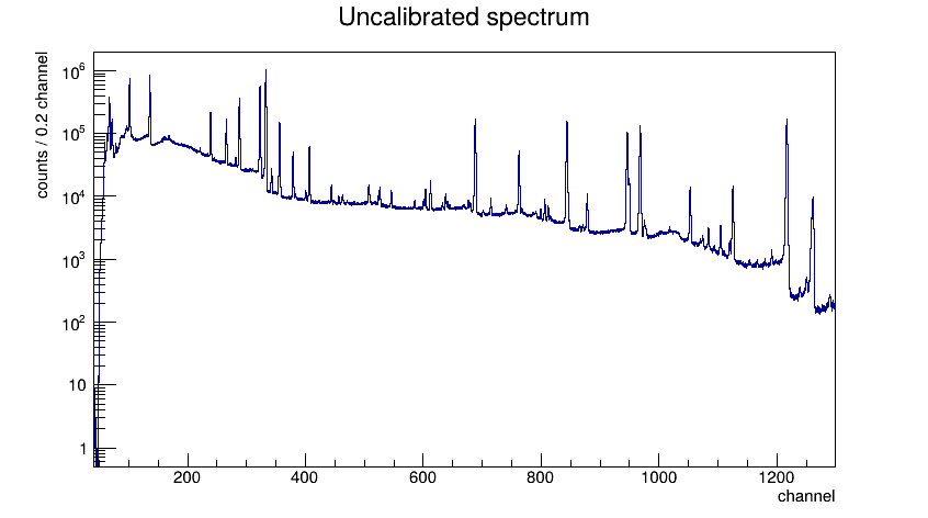
文件中包含 TH1F h0。横轴是未刻度的 channel,不应在 peak fit 前解释为 keV。完整谱用 log scale 显示,以便同时看到强峰和较弱峰。
import math
from array import array
import ROOT

%jsroot on
ROOT.gStyle.SetOptStat(0)

input_file = ROOT.TFile.Open("gamma.root", "READ")
if not input_file or input_file.IsZombie():
    raise OSError("cannot open gamma.root")

h_raw = input_file.Get("h0")
if not h_raw:
    raise KeyError("TH1 h0 is not present in gamma.root")

c_raw = ROOT.TCanvas("c_raw_py", "Raw gamma spectrum", 850, 500)
c_raw.SetLogy()
h_raw.SetTitle("Uncalibrated spectrum;channel;counts / 0.2 channel")
h_raw.GetXaxis().SetRangeUser(40, 1300)
h_raw.SetMinimum(0.5)
h_raw.Draw("hist")
c_raw.Draw()
c_raw.SaveAs("../coursework3.1/standard_source_spectrum.png")
//%jsroot on
#include "TBox.h"
#include "TCanvas.h"
#include "TFile.h"
#include "TF1.h"
#include "TFitResultPtr.h"
#include "TGraph.h"
#include "TGraphErrors.h"
#include "TH1.h"
#include "TH1D.h"
#include "TLegend.h"
#include "TLine.h"
#include "TMath.h"
#include "TPad.h"
#include "TStyle.h"
#include <algorithm>
#include <array>
#include <cmath>
#include <iomanip>
#include <iostream>
#include <stdexcept>
#include <string>
#include <vector>

gStyle->SetOptStat(0);

auto inputFile = TFile::Open("gamma.root", "READ");
if (!inputFile || inputFile->IsZombie()) {
    throw std::runtime_error("cannot open gamma.root");
}
auto hRaw = dynamic_cast<TH1*>(inputFile->Get("h0"));
if (!hRaw) {
    throw std::runtime_error("TH1 h0 is not present in gamma.root");
}

auto cRaw = new TCanvas("cRaw", "Raw gamma spectrum", 850, 500);
cRaw->SetLogy();
hRaw->SetTitle("Uncalibrated spectrum;channel;counts / 0.2 channel");
hRaw->GetXaxis()->SetRangeUser(40, 1300);
hRaw->SetMinimum(0.5);
hRaw->Draw("hist");
cRaw->Draw();
cRaw->SaveAs("../coursework3.1/standard_source_spectrum.png");
提取峰位与峰宽
对每条孤立参考线,先用峰两侧的 sidebands 拟合线性本底,估计初值;随后同时拟合 Gaussian 与本底,提取峰位、$\sigma$ 及其误差。下面的函数把作业 3.1 中的分步代码用于各条参考线。
approx_position = [101.7, 135.9, 239.1, 265.9, 288.1, 322.9,
                   332.7, 688.3, 762.7, 843.9, 968.3, 1217.1]
reference_energy = [80.9979, 121.7817, 244.6974, 276.3989,
                    302.8508, 344.2785, 356.0129, 778.9045,
                    867.378, 964.079, 1112.076, 1408.013]
half_width = [3.0, 3.0, 3.5, 3.5, 3.5, 3.5,
              3.5, 4.5, 6.0, 4.5, 5.0, 5.0]

def fit_peak_linear(hist, name, guess, width):
    xmin, xmax = guess - width, guess + width
    sideband_graph = ROOT.TGraphErrors()
    point = 0
    for bin_number in range(hist.FindBin(xmin), hist.FindBin(xmax) + 1):
        x = hist.GetBinCenter(bin_number)
        if abs(x - guess) < 0.5 * width:
            continue
        count = hist.GetBinContent(bin_number)
        sideband_graph.SetPoint(point, x, count)
        sideband_graph.SetPointError(point, 0.0, math.sqrt(max(count, 1.0)))
        point += 1

    seed = ROOT.TF1(
        name + "_seed", f"[0]+[1]*(x-{guess:.6f})", xmin, xmax
    )
    seed.SetParameters(hist.GetBinContent(hist.FindBin(xmin)), 0.0)
    sideband_graph.Fit(seed, "RSQN")
    height = max(hist.GetBinContent(hist.FindBin(guess)) - seed.GetParameter(0), 1.0)

    function = ROOT.TF1(
        name, f"gaus(0)+[3]+[4]*(x-{guess:.6f})", xmin, xmax
    )
    function.SetParNames("height", "mean", "sigma", "b0", "slope")
    function.SetParameters(
        height, guess, 0.8, seed.GetParameter(0), seed.GetParameter(1)
    )
    function.SetParLimits(0, 0.0, 10.0 * height)
    function.SetParLimits(1, guess - 2.0, guess + 2.0)
    function.SetParLimits(2, 0.2, 3.0)

    # L/I/R/S/Q/N: Poisson likelihood / bin integral / range /
    # fit result / quiet / do not attach or draw automatically.
    result = hist.Fit(function, "LIRSQN")

    background = ROOT.TF1(
        name + "_background", f"[0]+[1]*(x-{guess:.6f})", xmin, xmax
    )
    background.SetParameters(function.GetParameter(3), function.GetParameter(4))
    return {
        "function": function,
        "background": background,
        "status": int(result),
        "covariance_status": result.CovMatrixStatus(),
        "mean": function.GetParameter(1),
        "mean_error": function.GetParError(1),
        "sigma": abs(function.GetParameter(2)),
        "sigma_error": function.GetParError(2),
    }

peak_fits = [
    fit_peak_linear(h_raw, f"peak_{i}_py", guess, width)
    for i, (guess, width) in enumerate(zip(approx_position, half_width))
]

print(" E_ref (keV)    centroid       sigma    status/cov")
for energy, peak in zip(reference_energy, peak_fits):
    print(f" {energy:10.4f}  {peak['mean']:10.4f}  {peak['sigma']:9.4f}  "
          f"{peak['status']}/{peak['covariance_status']}")
const std::vector<double> approximatePosition = {
    101.7, 135.9, 239.1, 265.9, 288.1, 322.9,
    332.7, 688.3, 762.7, 843.9, 968.3, 1217.1};
const std::vector<double> referenceEnergy = {
    80.9979, 121.7817, 244.6974, 276.3989,
    302.8508, 344.2785, 356.0129, 778.9045,
    867.378, 964.079, 1112.076, 1408.013};
const std::vector<double> halfWidth = {
    3.0, 3.0, 3.5, 3.5, 3.5, 3.5,
    3.5, 4.5, 6.0, 4.5, 5.0, 5.0};

struct PeakFit {
    TF1* function;
    TF1* background;
    int status;
    int covarianceStatus;
    double mean;
    double meanError;
    double sigma;
    double sigmaError;
};

auto fitPeakLinear = [](TH1* hist, const std::string& name,
                        double guess, double width) {
    const double xmin = guess - width;
    const double xmax = guess + width;
    auto sidebandGraph = new TGraphErrors();
    int point = 0;
    for (int bin = hist->FindBin(xmin); bin <= hist->FindBin(xmax); ++bin) {
        const double x = hist->GetBinCenter(bin);
        if (std::abs(x - guess) < 0.5 * width) continue;
        const double count = hist->GetBinContent(bin);
        sidebandGraph->SetPoint(point, x, count);
        sidebandGraph->SetPointError(
            point, 0.0, std::sqrt(std::max(count, 1.0)));
        ++point;
    }

    const std::string backgroundFormula =
        "[0]+[1]*(x-" + std::to_string(guess) + ")";
    auto seed = new TF1((name + "_seed").c_str(), backgroundFormula.c_str(), xmin, xmax);
    seed->SetParameters(hist->GetBinContent(hist->FindBin(xmin)), 0.0);
    sidebandGraph->Fit(seed, "RSQN");
    const double height = std::max(
        hist->GetBinContent(hist->FindBin(guess)) - seed->GetParameter(0), 1.0);

    const std::string formula =
        "gaus(0)+[3]+[4]*(x-" + std::to_string(guess) + ")";
    auto function = new TF1(name.c_str(), formula.c_str(), xmin, xmax);
    function->SetParNames("height", "mean", "sigma", "b0", "slope");
    function->SetParameters(
        height, guess, 0.8, seed->GetParameter(0), seed->GetParameter(1));
    function->SetParLimits(0, 0.0, 10.0 * height);
    function->SetParLimits(1, guess - 2.0, guess + 2.0);
    function->SetParLimits(2, 0.2, 3.0);

    TFitResultPtr result = hist->Fit(function, "LIRSQN");
    auto background = new TF1(
        (name + "_background").c_str(), backgroundFormula.c_str(), xmin, xmax);
    background->SetParameters(function->GetParameter(3), function->GetParameter(4));

    PeakFit output;
    output.function = function;
    output.background = background;
    output.status = static_cast<int>(result);
    output.covarianceStatus = result->CovMatrixStatus();
    output.mean = function->GetParameter(1);
    output.meanError = function->GetParError(1);
    output.sigma = std::abs(function->GetParameter(2));
    output.sigmaError = function->GetParError(2);
    return output;
};

std::vector<PeakFit> peakFits;
std::vector<double> centroid;
std::vector<double> centroidError;
std::vector<double> peakSigma;
std::vector<double> peakSigmaError;

std::cout << " E_ref (keV)    centroid       sigma    status/cov\n";
for (std::size_t i = 0; i < approximatePosition.size(); ++i) {
    peakFits.push_back(fitPeakLinear(
        hRaw, "peak_" + std::to_string(i), approximatePosition[i], halfWidth[i]));
    const PeakFit& peak = peakFits.back();
    centroid.push_back(peak.mean);
    centroidError.push_back(peak.meanError);
    peakSigma.push_back(peak.sigma);
    peakSigmaError.push_back(peak.sigmaError);
    std::cout << std::fixed << std::setprecision(4)
              << std::setw(12) << referenceEnergy[i]
              << std::setw(12) << peak.mean
              << std::setw(11) << peak.sigma
              << std::setw(5) << peak.status << "/" << peak.covarianceStatus << "\n";
}
867.378 keV 峰与 residual
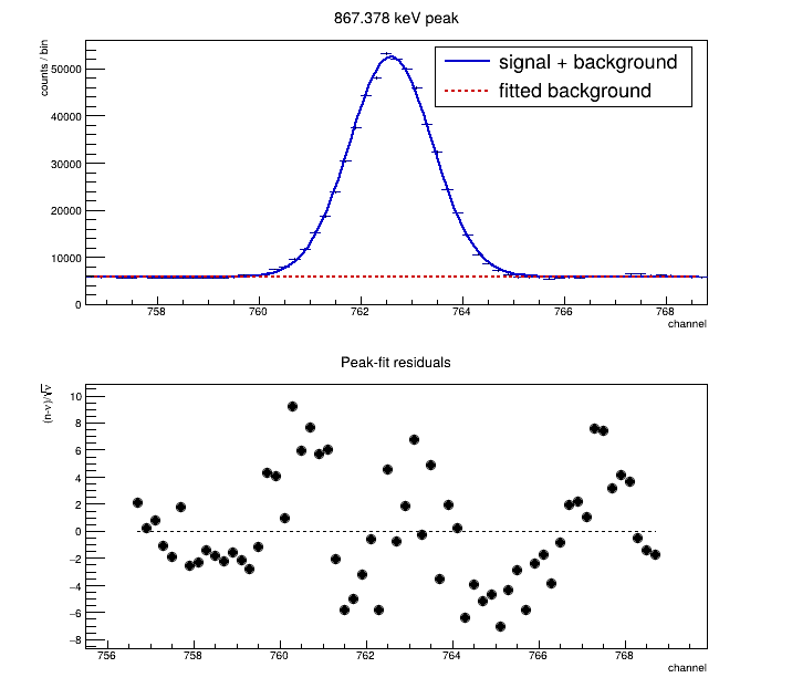
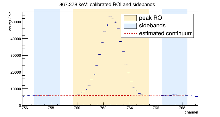
下面叠加数据、总模型和拟合本底,并绘制 Pearson residual,用于检查峰形与本底的描述。
def residual_graph(hist, function, xmin, xmax, name):
    graph = ROOT.TGraph()
    graph.SetName(name)
    point = 0
    for bin_number in range(hist.FindBin(xmin), hist.FindBin(xmax) + 1):
        low = hist.GetBinLowEdge(bin_number)
        width = hist.GetBinWidth(bin_number)
        expected = function.Integral(low, low + width) / width
        observed = hist.GetBinContent(bin_number)
        if expected > 0.0:
            graph.SetPoint(
                point, hist.GetBinCenter(bin_number),
                (observed - expected) / math.sqrt(expected)
            )
            point += 1
    return graph

example_index = 8
example_fit = peak_fits[example_index]
xmin867 = approx_position[example_index] - half_width[example_index]
xmax867 = approx_position[example_index] + half_width[example_index]
residual867 = residual_graph(
    h_raw, example_fit["function"], xmin867, xmax867, "res_867_py"
)

h_peak_view = h_raw.Clone("h_peak_867_view_py")
h_peak_view.GetXaxis().SetRangeUser(xmin867, xmax867)
h_peak_view.SetTitle("867.378 keV peak;channel;counts / bin")
h_peak_view.SetMinimum(0.0)
example_fit["function"].SetLineColor(ROOT.kBlue + 1)
example_fit["background"].SetLineColor(ROOT.kRed + 1)
example_fit["background"].SetLineStyle(2)

c_peak_model = ROOT.TCanvas("c_peak_model_py", "867.378 keV fit", 720, 650)
c_peak_model.Divide(1, 2)
c_peak_model.cd(1)
h_peak_view.Draw("E")
example_fit["function"].Draw("same")
example_fit["background"].Draw("same")
legend_peak = ROOT.TLegend(0.55, 0.70, 0.88, 0.88)
legend_peak.AddEntry(example_fit["function"], "signal + background", "l")
legend_peak.AddEntry(example_fit["background"], "fitted background", "l")
legend_peak.Draw()
c_peak_model.cd(2)
residual867.SetTitle("Peak-fit residuals;channel;(n-#nu)/#sqrt{#nu}")
residual867.SetMarkerStyle(20)
residual867.Draw("AP")
zero_peak = ROOT.TLine(xmin867, 0.0, xmax867, 0.0)
zero_peak.SetLineStyle(2)
zero_peak.Draw()
c_peak_model.Draw()
c_peak_model.SaveAs("../coursework3.1/fit_867_linear.png")
const std::size_t exampleIndex = 8;
const PeakFit& exampleFit = peakFits[exampleIndex];
const double xmin867 = approximatePosition[exampleIndex] - halfWidth[exampleIndex];
const double xmax867 = approximatePosition[exampleIndex] + halfWidth[exampleIndex];

auto residual867 = new TGraph();
int residualPoint = 0;
for (int bin = hRaw->FindBin(xmin867); bin <= hRaw->FindBin(xmax867); ++bin) {
    const double low = hRaw->GetBinLowEdge(bin);
    const double width = hRaw->GetBinWidth(bin);
    const double expected = exampleFit.function->Integral(low, low + width) / width;
    const double observed = hRaw->GetBinContent(bin);
    if (expected > 0.0) {
        residual867->SetPoint(
            residualPoint++, hRaw->GetBinCenter(bin),
            (observed - expected) / std::sqrt(expected));
    }
}

auto hPeakView = static_cast<TH1*>(hRaw->Clone("hPeak867View"));
hPeakView->GetXaxis()->SetRangeUser(xmin867, xmax867);
hPeakView->SetTitle("867.378 keV peak;channel;counts / bin");
hPeakView->SetMinimum(0.0);
exampleFit.function->SetLineColor(kBlue + 1);
exampleFit.background->SetLineColor(kRed + 1);
exampleFit.background->SetLineStyle(2);

auto cPeakModel = new TCanvas("cPeakModel", "867.378 keV fit", 720, 650);
cPeakModel->Divide(1, 2);
cPeakModel->cd(1);
hPeakView->Draw("E");
exampleFit.function->Draw("same");
exampleFit.background->Draw("same");
auto legendPeak = new TLegend(0.55, 0.70, 0.88, 0.88);
legendPeak->AddEntry(exampleFit.function, "signal + background", "l");
legendPeak->AddEntry(exampleFit.background, "fitted background", "l");
legendPeak->Draw();
cPeakModel->cd(2);
residual867->SetTitle("Peak-fit residuals;channel;(n-#nu)/#sqrt{#nu}");
residual867->SetMarkerStyle(20);
residual867->Draw("AP");
auto zeroPeak = new TLine(xmin867, 0.0, xmax867, 0.0);
zeroPeak->SetLineStyle(2);
zeroPeak->Draw();
cPeakModel->Draw();
cPeakModel->SaveAs("../coursework3.1/fit_867_linear.png");
能量刻度与 residual
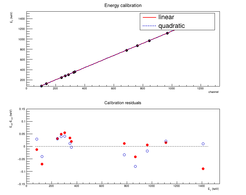
峰位误差放在 TGraphErrors 的横坐标误差中;参考能量的不确定度在本例尺度下忽略。一次和二次函数使用同一组峰位,通过 residual 比较两种刻度关系。
对这组数据,二次函数对最大绝对 residual 的改善很小,因此后续示例采用一次刻度。峰位的统计误差小于实际 residual,说明仅靠这些统计误差不足以解释刻度偏差,还应检查峰形、峰指认和刻度模型。
centroid = [peak["mean"] for peak in peak_fits]
centroid_error = [peak["mean_error"] for peak in peak_fits]
zero_error = [0.0] * len(reference_energy)
g_calibration = ROOT.TGraphErrors(
    len(centroid), array("d", centroid), array("d", reference_energy),
    array("d", centroid_error), array("d", zero_error)
)
g_calibration.SetTitle("Energy calibration;channel;E_{#gamma} (keV)")
g_calibration.SetMarkerStyle(20)

cal_linear = ROOT.TF1("cal_linear_py", "pol1", 90, 1230)
cal_quadratic = ROOT.TF1("cal_quadratic_py", "pol2", 90, 1230)
cal_linear.SetParameters(-40.0, 1.19)
cal_quadratic.SetParameters(-40.0, 1.19, 0.0)
cal_linear.SetLineColor(ROOT.kRed)
cal_quadratic.SetLineColor(ROOT.kBlue + 1)
cal_quadratic.SetLineStyle(2)

# F forces the general minimizer so the TGraphErrors x errors are used.
result_cal_linear = g_calibration.Fit(cal_linear, "RFSQN")
result_cal_quadratic = g_calibration.Fit(cal_quadratic, "RFSQN")

residual_cal_linear = ROOT.TGraph()
residual_cal_quadratic = ROOT.TGraph()
for i, (channel, energy) in enumerate(zip(centroid, reference_energy)):
    residual_cal_linear.SetPoint(i, energy, energy - cal_linear.Eval(channel))
    residual_cal_quadratic.SetPoint(i, energy, energy - cal_quadratic.Eval(channel))

c_energy = ROOT.TCanvas("c_energy_py", "Energy calibration", 850, 700)
c_energy.Divide(1, 2)
c_energy.cd(1)
g_calibration.Draw("AP")
cal_linear.Draw("same")
cal_quadratic.Draw("same")
legend_energy = ROOT.TLegend(0.57, 0.70, 0.88, 0.88)
legend_energy.AddEntry(cal_linear, "linear", "l")
legend_energy.AddEntry(cal_quadratic, "quadratic", "l")
legend_energy.Draw()
c_energy.cd(2)
residual_cal_linear.SetTitle(
    "Calibration residuals;E_{#gamma} (keV);E_{ref}-E_{cal} (keV)"
)
residual_cal_linear.SetMarkerStyle(20)
residual_cal_linear.SetMarkerColor(ROOT.kRed)
residual_cal_linear.SetMinimum(-0.15)
residual_cal_linear.SetMaximum(0.15)
residual_cal_quadratic.SetMarkerStyle(24)
residual_cal_quadratic.SetMarkerColor(ROOT.kBlue + 1)
residual_cal_linear.Draw("AP")
residual_cal_quadratic.Draw("P same")
zero_energy = ROOT.TLine(70.0, 0.0, 1450.0, 0.0)
zero_energy.SetLineStyle(2)
zero_energy.Draw()
c_energy.Draw()
c_energy.SaveAs("../coursework3.1/reference_energy_calibration.png")

max_residual_linear = max(
    abs(energy - cal_linear.Eval(channel))
    for channel, energy in zip(centroid, reference_energy)
)
max_residual_quadratic = max(
    abs(energy - cal_quadratic.Eval(channel))
    for channel, energy in zip(centroid, reference_energy)
)
print(f"linear status = {int(result_cal_linear)}, "
      f"E = {cal_linear.GetParameter(0):.6f} "
      f"+ {cal_linear.GetParameter(1):.9f} ch, "
      f"max |residual| = {max_residual_linear:.4f} keV")
print(f"quadratic status = {int(result_cal_quadratic)}, "
      f"a2 = {cal_quadratic.GetParameter(2):.3e}, "
      f"max |residual| = {max_residual_quadratic:.4f} keV")

calibration = cal_linear
std::vector<double> zeroError(referenceEnergy.size(), 0.0);
auto gCalibration = new TGraphErrors(
    centroid.size(), centroid.data(), referenceEnergy.data(),
    centroidError.data(), zeroError.data());
gCalibration->SetTitle("Energy calibration;channel;E_{#gamma} (keV)");
gCalibration->SetMarkerStyle(20);

auto calLinear = new TF1("calLinear", "pol1", 90, 1230);
auto calQuadratic = new TF1("calQuadratic", "pol2", 90, 1230);
calLinear->SetParameters(-40.0, 1.19);
calQuadratic->SetParameters(-40.0, 1.19, 0.0);
calLinear->SetLineColor(kRed);
calQuadratic->SetLineColor(kBlue + 1);
calQuadratic->SetLineStyle(2);

TFitResultPtr resultCalLinear = gCalibration->Fit(calLinear, "RFSQN");
TFitResultPtr resultCalQuadratic = gCalibration->Fit(calQuadratic, "RFSQN");

auto residualCalLinear = new TGraph();
auto residualCalQuadratic = new TGraph();
for (std::size_t i = 0; i < centroid.size(); ++i) {
    residualCalLinear->SetPoint(
        i, referenceEnergy[i], referenceEnergy[i] - calLinear->Eval(centroid[i]));
    residualCalQuadratic->SetPoint(
        i, referenceEnergy[i], referenceEnergy[i] - calQuadratic->Eval(centroid[i]));
}

auto cEnergy = new TCanvas("cEnergy", "Energy calibration", 850, 700);
cEnergy->Divide(1, 2);
cEnergy->cd(1);
gCalibration->Draw("AP");
calLinear->Draw("same");
calQuadratic->Draw("same");
auto legendEnergy = new TLegend(0.57, 0.70, 0.88, 0.88);
legendEnergy->AddEntry(calLinear, "linear", "l");
legendEnergy->AddEntry(calQuadratic, "quadratic", "l");
legendEnergy->Draw();
cEnergy->cd(2);
residualCalLinear->SetTitle(
    "Calibration residuals;E_{#gamma} (keV);E_{ref}-E_{cal} (keV)");
residualCalLinear->SetMarkerStyle(20);
residualCalLinear->SetMarkerColor(kRed);
residualCalLinear->SetMinimum(-0.15);
residualCalLinear->SetMaximum(0.15);
residualCalQuadratic->SetMarkerStyle(24);
residualCalQuadratic->SetMarkerColor(kBlue + 1);
residualCalLinear->Draw("AP");
residualCalQuadratic->Draw("P same");
auto zeroEnergy = new TLine(70.0, 0.0, 1450.0, 0.0);
zeroEnergy->SetLineStyle(2);
zeroEnergy->Draw();
cEnergy->Draw();
cEnergy->SaveAs("../coursework3.1/reference_energy_calibration.png");

double maxResidualLinear = 0.0;
double maxResidualQuadratic = 0.0;
for (std::size_t i = 0; i < centroid.size(); ++i) {
    maxResidualLinear = std::max(
        maxResidualLinear,
        std::abs(referenceEnergy[i] - calLinear->Eval(centroid[i])));
    maxResidualQuadratic = std::max(
        maxResidualQuadratic,
        std::abs(referenceEnergy[i] - calQuadratic->Eval(centroid[i])));
}
std::cout << std::fixed << std::setprecision(6)
          << "linear status = " << static_cast<int>(resultCalLinear)
          << ", E = " << calLinear->GetParameter(0)
          << " + " << std::setprecision(9) << calLinear->GetParameter(1)
          << " ch, max |residual| = " << std::setprecision(4)
          << maxResidualLinear << " keV\n"
          << "quadratic status = " << static_cast<int>(resultCalQuadratic)
          << ", a2 = " << std::scientific << calQuadratic->GetParameter(2)
          << std::fixed << ", max |residual| = " << maxResidualQuadratic
          << " keV" << std::endl;

TF1* calibration = calLinear;
生成刻度后的能谱
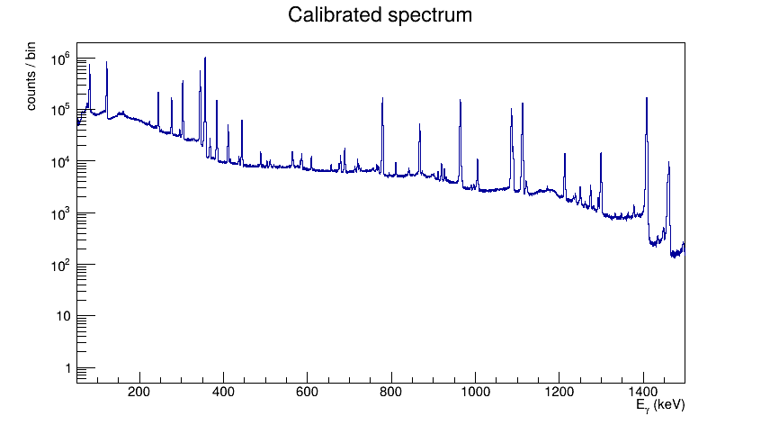
本例采用一次刻度,保持原 histogram 的 bin 数,把横轴上下限换算为能量,并逐 bin 复制计数和误差。变换前后的总计数应一致。
energy_min = calibration.Eval(h_raw.GetXaxis().GetXmin())
energy_max = calibration.Eval(h_raw.GetXaxis().GetXmax())
h_calibrated = ROOT.TH1D(
    "h_calibrated_py", "Calibrated spectrum;E_{#gamma} (keV);counts / bin",
    h_raw.GetNbinsX(), energy_min, energy_max
)
for bin_number in range(0, h_calibrated.GetNbinsX() + 2):
    h_calibrated.SetBinContent(bin_number, h_raw.GetBinContent(bin_number))
    h_calibrated.SetBinError(bin_number, h_raw.GetBinError(bin_number))
h_calibrated.SetEntries(h_raw.GetEntries())

c_calibrated = ROOT.TCanvas("c_calibrated_py", "Calibrated spectrum", 850, 500)
c_calibrated.SetLogy()
h_calibrated.SetMinimum(0.5)
h_calibrated.GetXaxis().SetRangeUser(50, 1500)
h_calibrated.Draw("hist")
c_calibrated.Draw()
c_calibrated.SaveAs("../coursework3.1/reference_calibrated_spectrum.png")

raw_counts = h_raw.Integral(0, h_raw.GetNbinsX() + 1)
mapped_counts = h_calibrated.Integral(0, h_calibrated.GetNbinsX() + 1)
print(f"mapped counts / input counts = {mapped_counts:.0f} / {raw_counts:.0f}")
const double energyMin = calibration->Eval(hRaw->GetXaxis()->GetXmin());
const double energyMax = calibration->Eval(hRaw->GetXaxis()->GetXmax());
auto hCalibrated = new TH1D(
    "hCalibrated", "Calibrated spectrum;E_{#gamma} (keV);counts / bin",
    hRaw->GetNbinsX(), energyMin, energyMax);
for (int bin = 0; bin <= hCalibrated->GetNbinsX() + 1; ++bin) {
    hCalibrated->SetBinContent(bin, hRaw->GetBinContent(bin));
    hCalibrated->SetBinError(bin, hRaw->GetBinError(bin));
}
hCalibrated->SetEntries(hRaw->GetEntries());

auto cCalibrated = new TCanvas(
    "cCalibrated", "Calibrated spectrum", 850, 500);
cCalibrated->SetLogy();
hCalibrated->SetMinimum(0.5);
hCalibrated->GetXaxis()->SetRangeUser(50, 1500);
hCalibrated->Draw("hist");
cCalibrated->Draw();
cCalibrated->SaveAs("../coursework3.1/reference_calibrated_spectrum.png");

const double rawCounts = hRaw->Integral(0, hRaw->GetNbinsX() + 1);
const double mappedCounts = hCalibrated->Integral(0, hCalibrated->GetNbinsX() + 1);
std::cout << std::fixed << std::setprecision(0)
          << "mapped counts / input counts = " << mappedCounts
          << " / " << rawCounts << std::endl;
FWHM 随能量的变化
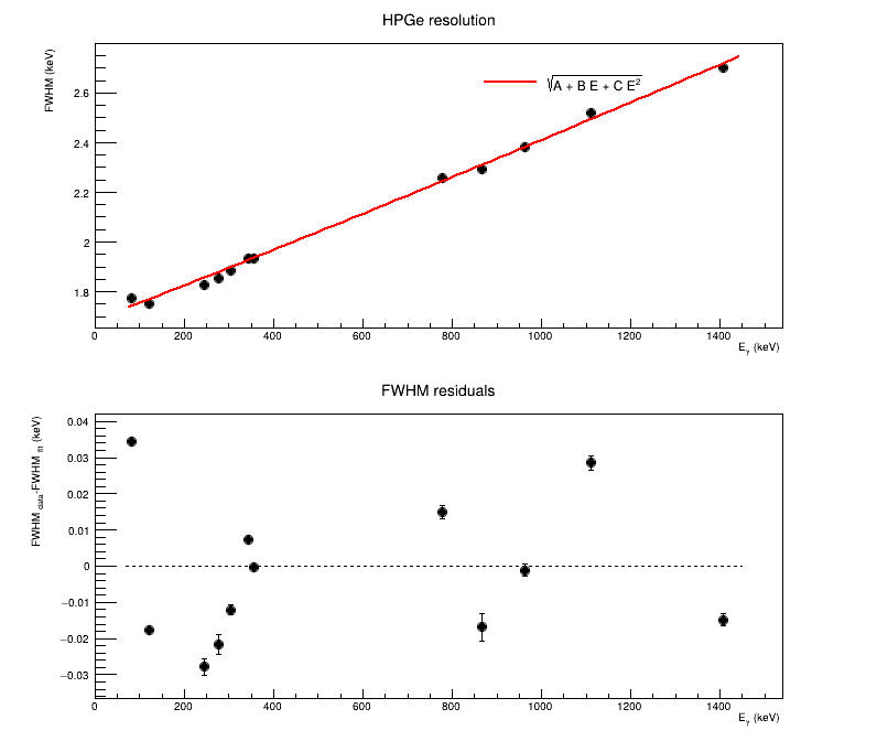
各 peak 的 $\sigma_{ch}$ 由所选刻度曲线的局部导数换算为 $\sigma_E$,再由 $FWHM=2.355\sigma_E$ 得到 FWHM。当载流子统计涨落占主导时,$\sigma_E^2\propto E$,因此 $\sigma_E$ 和 FWHM 均正比于 $\sqrt{E}$。实际探测器中,电子学噪声、载流子统计和电荷收集等近似独立的贡献在方差层面相加,因此采用
$$FWHM(E)=\sqrt{A+BE+CE^2}$$
拟合中限定 $A$、$B$、$C$ 非负,使三项分别表示非负的方差贡献。该曲线在有限能区内可能看起来接近直线,但不代表 FWHM 一般与能量成线性关系。误差棒只传播 local fit 对 $\sigma$ 的统计误差;刻度函数和 peak-shape model 的系统效应未包含。
fwhm = []
fwhm_error = []
for channel, peak in zip(centroid, peak_fits):
    derivative = calibration.GetParameter(1)
    factor = 2.0 * math.sqrt(2.0 * math.log(2.0)) * abs(derivative)
    fwhm.append(factor * peak["sigma"])
    fwhm_error.append(factor * peak["sigma_error"])

g_width = ROOT.TGraphErrors(
    len(reference_energy), array("d", reference_energy), array("d", fwhm),
    array("d", zero_error), array("d", fwhm_error)
)
g_width.SetTitle("HPGe resolution;E_{#gamma} (keV);FWHM (keV)")
g_width.SetMarkerStyle(20)

width_model = ROOT.TF1(
    "width_model_py", "sqrt([0]+[1]*x+[2]*x*x)", 70, 1450
)
width_model.SetParNames("A", "B", "C")
width_model.SetParameters(2.8, 0.0023, 6.5e-7)
width_model.SetParLimits(0, 0.0, 10.0)
width_model.SetParLimits(1, 0.0, 0.1)
width_model.SetParLimits(2, 0.0, 1.0e-4)
width_model.SetLineColor(ROOT.kRed)
result_width = g_width.Fit(width_model, "RSQN")

residual_width = ROOT.TGraphErrors()
for i, (energy, value, error) in enumerate(
    zip(reference_energy, fwhm, fwhm_error)
):
    residual_width.SetPoint(i, energy, value - width_model.Eval(energy))
    residual_width.SetPointError(i, 0.0, error)

c_width = ROOT.TCanvas("c_width_py", "FWHM calibration", 800, 700)
c_width.Divide(1, 2)
c_width.cd(1)
g_width.Draw("AP")
width_model.Draw("same")
legend_width = ROOT.TLegend(0.54, 0.74, 0.88, 0.84)
legend_width.AddEntry(width_model, "#sqrt{A + B E + C E^{2}}", "l")
legend_width.SetTextSize(0.040)
legend_width.SetBorderSize(0)
legend_width.SetFillStyle(0)
legend_width.Draw()
c_width.cd(2)
residual_width.SetTitle(
    "FWHM residuals;E_{#gamma} (keV);FWHM_{data}-FWHM_{fit} (keV)"
)
residual_width.SetMarkerStyle(20)
residual_width.Draw("AP")
zero_width = ROOT.TLine(70.0, 0.0, 1450.0, 0.0)
zero_width.SetLineStyle(2)
zero_width.Draw()
c_width.Draw()
c_width.SaveAs("../coursework3.1/reference_fwhm.png")

print(f"FWHM fit status = {int(result_width)}")
print(f"A = {width_model.GetParameter(0):.6f}, "
      f"B = {width_model.GetParameter(1):.8f}, "
      f"C = {width_model.GetParameter(2):.10f}")
std::vector<double> fwhm;
std::vector<double> fwhmError;
for (std::size_t i = 0; i < peakSigma.size(); ++i) {
    const double derivative = calibration->GetParameter(1);
    const double factor = 2.0 * std::sqrt(2.0 * std::log(2.0))
        * std::abs(derivative);
    fwhm.push_back(factor * peakSigma[i]);
    fwhmError.push_back(factor * peakSigmaError[i]);
}

auto gWidth = new TGraphErrors(
    referenceEnergy.size(), referenceEnergy.data(), fwhm.data(),
    zeroError.data(), fwhmError.data());
gWidth->SetTitle("HPGe resolution;E_{#gamma} (keV);FWHM (keV)");
gWidth->SetMarkerStyle(20);

auto widthModel = new TF1(
    "widthModel", "sqrt([0]+[1]*x+[2]*x*x)", 70, 1450);
widthModel->SetParNames("A", "B", "C");
widthModel->SetParameters(2.8, 0.0023, 6.5e-7);
widthModel->SetParLimits(0, 0.0, 10.0);
widthModel->SetParLimits(1, 0.0, 0.1);
widthModel->SetParLimits(2, 0.0, 1.0e-4);
widthModel->SetLineColor(kRed);
TFitResultPtr resultWidth = gWidth->Fit(widthModel, "RSQN");

auto residualWidth = new TGraphErrors();
for (std::size_t i = 0; i < referenceEnergy.size(); ++i) {
    residualWidth->SetPoint(
        i, referenceEnergy[i], fwhm[i] - widthModel->Eval(referenceEnergy[i]));
    residualWidth->SetPointError(i, 0.0, fwhmError[i]);
}

auto cWidth = new TCanvas("cWidth", "FWHM calibration", 800, 700);
cWidth->Divide(1, 2);
cWidth->cd(1);
gWidth->Draw("AP");
widthModel->Draw("same");
auto legendWidth = new TLegend(0.54, 0.74, 0.88, 0.84);
legendWidth->AddEntry(widthModel, "#sqrt{A + B E + C E^{2}}", "l");
legendWidth->SetTextSize(0.040);
legendWidth->SetBorderSize(0);
legendWidth->SetFillStyle(0);
legendWidth->Draw();
cWidth->cd(2);
residualWidth->SetTitle(
    "FWHM residuals;E_{#gamma} (keV);FWHM_{data}-FWHM_{fit} (keV)");
residualWidth->SetMarkerStyle(20);
residualWidth->Draw("AP");
auto zeroWidth = new TLine(70.0, 0.0, 1450.0, 0.0);
zeroWidth->SetLineStyle(2);
zeroWidth->Draw();
cWidth->Draw();
cWidth->SaveAs("../coursework3.1/reference_fwhm.png");

std::cout << "FWHM fit status = " << static_cast<int>(resultWidth) << "\n"
          << std::fixed << std::setprecision(5)
          << "A = " << widthModel->GetParameter(0)
          << ", B = " << std::setprecision(8) << widthModel->GetParameter(1)
          << ", C = " << std::setprecision(10) << widthModel->GetParameter(2)
          << std::endl;
用 ROI summation 提取净峰面积
对每条参考线,calibration.GetX 用已知 $E_\gamma$ 反求 channel,calibration.Derivative 把 width_model 给出的 keV FWHM 换成 channel。按此设置 ROI 与 sidebands,再累加计数、扣除本底并计算净面积误差。
def integrate_peak(hist, center, fwhm):
    bounds = {
        "left": (center - 3.0*fwhm, center - 2.0*fwhm),
        "roi": (center - 1.5*fwhm, center + 1.5*fwhm),
        "right": (center + 2.0*fwhm, center + 3.0*fwhm),
    }
    counts = {"left": 0.0, "roi": 0.0, "right": 0.0}
    bins = {"left": 0, "roi": 0, "right": 0}
    for bin_number in range(
        hist.FindBin(bounds["left"][0]), hist.FindBin(bounds["right"][1]) + 1
    ):
        x = hist.GetBinCenter(bin_number)
        for region in ("left", "roi", "right"):
            low, high = bounds[region]
            if low <= x <= high:
                counts[region] += hist.GetBinContent(bin_number)
                bins[region] += 1
                break

    gross = counts["roi"]
    weight_left = 0.5 * bins["roi"] / bins["left"]
    weight_right = 0.5 * bins["roi"] / bins["right"]
    background = weight_left*counts["left"] + weight_right*counts["right"]
    net = gross - background
    variance = (
        gross + weight_left**2*counts["left"]
        + weight_right**2*counts["right"]
    )
    return {
        "center": center, "fwhm": fwhm, "bounds": bounds,
        "counts": counts, "bins": bins, "gross": gross,
        "background_count": background, "net": net,
        "net_error": math.sqrt(variance),
    }

peak_areas = []
peak_net = []
peak_net_error = []
for energy in reference_energy:
    center = calibration.GetX(energy, 40.0, 1300.0)
    kev_per_channel = abs(calibration.Derivative(center))
    fwhm_channel = width_model.Eval(energy) / kev_per_channel
    area = integrate_peak(h_raw, center, fwhm_channel)
    peak_areas.append(area)
    peak_net.append(area["net"])
    peak_net_error.append(area["net_error"])

print(" E_ref (keV)  ROI center   FWHM_ch       gross  background        net")
for energy, area in zip(reference_energy, peak_areas):
    print(f" {energy:10.4f}  {area['center']:10.4f}  {area['fwhm']:8.4f}  "
          f"{area['gross']:10.0f}  {area['background_count']:10.1f}  "
          f"{area['net']:10.1f}")

# Show the regions used for the 867.378 keV area.
example_index = 8
example_area = peak_areas[example_index]
bounds = example_area["bounds"]
left_rate = example_area["counts"]["left"] / example_area["bins"]["left"]
right_rate = example_area["counts"]["right"] / example_area["bins"]["right"]
left_center = 0.5 * sum(bounds["left"])
right_center = 0.5 * sum(bounds["right"])
continuum = ROOT.TF1(
    "continuum_867_py", "[0]+[1]*(x-[2])",
    bounds["left"][0], bounds["right"][1]
)
continuum.SetParameters(
    left_rate, (right_rate-left_rate)/(right_center-left_center), left_center
)
continuum.SetLineColor(ROOT.kRed + 1)
continuum.SetLineStyle(2)

c_integration = ROOT.TCanvas("c_integration_py", "867 ROI", 760, 430)
h_integration = h_raw.Clone("h_integration_867_py")
h_integration.GetXaxis().SetRangeUser(
    bounds["left"][0] - 0.4*example_area["fwhm"],
    bounds["right"][1] + 0.4*example_area["fwhm"]
)
h_integration.SetTitle("867.378 keV: calibrated ROI and sidebands;channel;counts / bin")
h_integration.SetMinimum(0.0)
h_integration.Draw("E")
ymax = 1.08 * h_integration.GetMaximum()
left_box = ROOT.TBox(bounds["left"][0], 0.0, bounds["left"][1], ymax)
roi_box = ROOT.TBox(bounds["roi"][0], 0.0, bounds["roi"][1], ymax)
right_box = ROOT.TBox(bounds["right"][0], 0.0, bounds["right"][1], ymax)
for box in (left_box, right_box):
    box.SetFillColorAlpha(ROOT.kAzure - 9, 0.28)
    box.Draw("same")
roi_box.SetFillColorAlpha(ROOT.kOrange - 2, 0.25)
roi_box.Draw("same")
h_integration.Draw("E same")
continuum.Draw("same")
legend_integration = ROOT.TLegend(0.55, 0.68, 0.88, 0.88)
legend_integration.AddEntry(roi_box, "peak ROI", "f")
legend_integration.AddEntry(left_box, "sidebands", "f")
legend_integration.AddEntry(continuum, "estimated continuum", "l")
legend_integration.Draw()
c_integration.Draw()
c_integration.SaveAs("../coursework3.1/roi_867_integration.png")
struct PeakArea {
    double center;
    double fwhm;
    double leftLow;
    double leftHigh;
    double roiLow;
    double roiHigh;
    double rightLow;
    double rightHigh;
    double leftCounts;
    double rightCounts;
    double gross;
    double background;
    double net;
    double netError;
    int leftBins;
    int rightBins;
    int roiBins;
};

auto integratePeak = [](TH1* hist, double center, double fwhm) {
    PeakArea area{};
    area.center = center;
    area.fwhm = fwhm;
    area.leftLow = center - 3.0*fwhm;
    area.leftHigh = center - 2.0*fwhm;
    area.roiLow = center - 1.5*fwhm;
    area.roiHigh = center + 1.5*fwhm;
    area.rightLow = center + 2.0*fwhm;
    area.rightHigh = center + 3.0*fwhm;

    for (int bin = hist->FindBin(area.leftLow);
         bin <= hist->FindBin(area.rightHigh); ++bin) {
        const double x = hist->GetBinCenter(bin);
        const double count = hist->GetBinContent(bin);
        if (x >= area.leftLow && x <= area.leftHigh) {
            area.leftCounts += count;
            ++area.leftBins;
        } else if (x >= area.roiLow && x <= area.roiHigh) {
            area.gross += count;
            ++area.roiBins;
        } else if (x >= area.rightLow && x <= area.rightHigh) {
            area.rightCounts += count;
            ++area.rightBins;
        }
    }

    const double leftWeight = 0.5*area.roiBins/area.leftBins;
    const double rightWeight = 0.5*area.roiBins/area.rightBins;
    area.background = leftWeight*area.leftCounts + rightWeight*area.rightCounts;
    area.net = area.gross - area.background;
    const double variance = area.gross
        + leftWeight*leftWeight*area.leftCounts
        + rightWeight*rightWeight*area.rightCounts;
    area.netError = std::sqrt(variance);
    return area;
};

std::vector<PeakArea> peakAreas;
std::vector<double> peakNet;
std::vector<double> peakNetError;
for (double energy : referenceEnergy) {
    const double center = calibration->GetX(energy, 40.0, 1300.0);
    const double kevPerChannel = std::abs(calibration->Derivative(center));
    const double fwhmChannel = widthModel->Eval(energy) / kevPerChannel;
    peakAreas.push_back(integratePeak(hRaw, center, fwhmChannel));
    peakNet.push_back(peakAreas.back().net);
    peakNetError.push_back(peakAreas.back().netError);
}

std::cout << " E_ref (keV)  ROI center   FWHM_ch       gross  background        net\n";
for (std::size_t i = 0; i < referenceEnergy.size(); ++i) {
    const PeakArea& area = peakAreas[i];
    std::cout << std::fixed << std::setprecision(4)
              << std::setw(12) << referenceEnergy[i]
              << std::setw(12) << area.center
              << std::setw(10) << area.fwhm
              << std::setw(12) << std::setprecision(0) << area.gross
              << std::setw(12) << std::setprecision(1) << area.background
              << std::setw(12) << area.net << "\n";
}

// Show the regions used for the 867.378 keV area.
const std::size_t areaExampleIndex = 8;
const PeakArea& exampleArea = peakAreas[areaExampleIndex];
const double leftRate = exampleArea.leftCounts/exampleArea.leftBins;
const double rightRate = exampleArea.rightCounts/exampleArea.rightBins;
const double leftCenter = 0.5*(exampleArea.leftLow + exampleArea.leftHigh);
const double rightCenter = 0.5*(exampleArea.rightLow + exampleArea.rightHigh);
auto continuum = new TF1(
    "continuum867", "[0]+[1]*(x-[2])",
    exampleArea.leftLow, exampleArea.rightHigh);
continuum->SetParameters(
    leftRate, (rightRate-leftRate)/(rightCenter-leftCenter), leftCenter);
continuum->SetLineColor(kRed + 1);
continuum->SetLineStyle(2);

auto cIntegration = new TCanvas("cIntegration", "867 ROI", 760, 430);
auto hIntegration = static_cast<TH1*>(hRaw->Clone("hIntegration867"));
hIntegration->GetXaxis()->SetRangeUser(
    exampleArea.leftLow - 0.4*exampleArea.fwhm,
    exampleArea.rightHigh + 0.4*exampleArea.fwhm);
hIntegration->SetTitle("867.378 keV: calibrated ROI and sidebands;channel;counts / bin");
hIntegration->SetMinimum(0.0);
hIntegration->Draw("E");
const double ymax = 1.08*hIntegration->GetMaximum();
auto leftBox = new TBox(exampleArea.leftLow, 0.0, exampleArea.leftHigh, ymax);
auto roiBox = new TBox(exampleArea.roiLow, 0.0, exampleArea.roiHigh, ymax);
auto rightBox = new TBox(exampleArea.rightLow, 0.0, exampleArea.rightHigh, ymax);
leftBox->SetFillColorAlpha(kAzure - 9, 0.28);
rightBox->SetFillColorAlpha(kAzure - 9, 0.28);
roiBox->SetFillColorAlpha(kOrange - 2, 0.25);
leftBox->Draw("same");
rightBox->Draw("same");
roiBox->Draw("same");
hIntegration->Draw("E same");
continuum->Draw("same");
auto legendIntegration = new TLegend(0.55, 0.68, 0.88, 0.88);
legendIntegration->AddEntry(roiBox, "peak ROI", "f");
legendIntegration->AddEntry(leftBox, "sidebands", "f");
legendIntegration->AddEntry(continuum, "estimated continuum", "l");
legendIntegration->Draw();
cIntegration->Draw();
cIntegration->SaveAs("../coursework3.1/roi_867_integration.png");
Apparent full-energy peak efficiency
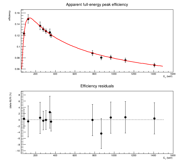
每个效率点使用 ROI summation 得到的 $N_{\rm net}$。图中误差棒包含计数误差、gamma emission probability 和源活度误差。同一源的活度误差相关,本例曲线拟合的权重只采用计数和发射概率的误差,活度误差作为共同的归一化误差单独考虑。
$$ \varepsilon(E)=\exp\!\left[p_0+p_1u+p_2u^2-p_3(100\ \mathrm{keV}/E)^3\right], \qquad u=\ln(E/100\ \mathrm{keV}). $$
结果采用线性横、纵坐标,并显示相对 residual。最低参考线为 81 keV,曲线在更低能区没有数据约束。数据未提供 dead-time 与 true-coincidence-summing correction,因此结果标为 apparent efficiency。这里暂把 7442 s 作为 live time;若采集记录区分 real time 与 live time,应使用后者。
nuclide = ["Ba", "Eu", "Eu", "Ba", "Ba", "Eu",
           "Ba", "Eu", "Eu", "Eu", "Eu", "Eu"]
gamma_probability = [0.3406, 0.2841, 0.0755, 0.07164, 0.1833, 0.2659,
                     0.6205, 0.1293, 0.0423, 0.1451, 0.1367, 0.2087]
gamma_probability_rel_error = [0.008, 0.005, 0.006, 0.004, 0.004, 0.005,
                               0.004, 0.006, 0.007, 0.005, 0.006, 0.005]

elapsed_days = 5522.0
live_time = 7442.0
activity_reference = {"Eu": 40.9e3, "Ba": 42.2e3}
half_life_days = {"Eu": 13.517 * 365.25, "Ba": 3849.3}
activity_rel_error = {"Eu": 0.05, "Ba": 0.03}
activity = {
    key: activity_reference[key] * 2.0**(-elapsed_days / half_life_days[key])
    for key in activity_reference
}

efficiency = []
efficiency_error = []
efficiency_fit_error = []
for area, isotope, probability, probability_rel_error in zip(
    peak_areas, nuclide, gamma_probability, gamma_probability_rel_error
):
    value = area["net"] / (activity[isotope] * probability * live_time)
    count_rel_error = area["net_error"] / area["net"]
    uncorrelated_rel_error = math.sqrt(
        count_rel_error**2 + probability_rel_error**2
    )
    total_rel_error = math.sqrt(
        uncorrelated_rel_error**2 + activity_rel_error[isotope]**2
    )
    efficiency.append(value)
    efficiency_fit_error.append(value * uncorrelated_rel_error)
    efficiency_error.append(value * total_rel_error)

g_efficiency = ROOT.TGraphErrors(
    len(reference_energy), array("d", reference_energy), array("d", efficiency),
    array("d", zero_error), array("d", efficiency_error)
)
g_efficiency_fit = ROOT.TGraphErrors(
    len(reference_energy), array("d", reference_energy), array("d", efficiency),
    array("d", zero_error), array("d", efficiency_fit_error)
)
g_efficiency.SetTitle(
    "Apparent full-energy peak efficiency;E_{#gamma} (keV);efficiency"
)
g_efficiency.SetMarkerStyle(20)

efficiency_model = ROOT.TF1(
    "efficiency_model_py",
    "exp([0]+[1]*log(x/100.0)+[2]*pow(log(x/100.0),2)"
    "-[3]*pow(100.0/x,3))", 50, 1500
)
efficiency_model.SetParNames("p0", "p1", "p2", "low-energy absorption")
efficiency_model.SetParameters(-1.8, -0.2, -0.05, 0.2)
efficiency_model.SetParLimits(3, 0.0, 10.0)
efficiency_model.SetLineColor(ROOT.kRed)
result_efficiency = g_efficiency_fit.Fit(efficiency_model, "RSQN")

residual_efficiency = ROOT.TGraphErrors()
for i, (energy, value, error) in enumerate(
    zip(reference_energy, efficiency, efficiency_error)
):
    fitted = efficiency_model.Eval(energy)
    residual_efficiency.SetPoint(i, energy, 100.0 * (value - fitted) / fitted)
    residual_efficiency.SetPointError(i, 0.0, 100.0 * error / fitted)

c_efficiency = ROOT.TCanvas("c_efficiency_py", "Efficiency", 800, 700)
c_efficiency.Divide(1, 2)
c_efficiency.cd(1)
ROOT.gPad.SetLogx(0)
ROOT.gPad.SetLogy(0)
g_efficiency.Draw("AP")
g_efficiency.GetXaxis().SetLimits(50.0, 1600.0)
efficiency_model.Draw("same")
c_efficiency.cd(2)
ROOT.gPad.SetLogx(0)
residual_efficiency.SetTitle(
    "Efficiency residuals;E_{#gamma} (keV);(data-fit)/fit (%)"
)
residual_efficiency.SetMarkerStyle(20)
residual_efficiency.Draw("AP")
residual_efficiency.GetXaxis().SetLimits(50.0, 1600.0)
zero_efficiency = ROOT.TLine(50.0, 0.0, 1500.0, 0.0)
zero_efficiency.SetLineStyle(2)
zero_efficiency.Draw()
c_efficiency.Draw()
c_efficiency.SaveAs("../coursework3.1/reference_efficiency.png")

print(f"activity at measurement: Eu-152 = {activity['Eu']:.1f} Bq, "
      f"Ba-133 = {activity['Ba']:.1f} Bq")
print(f"efficiency fit status/covariance status = "
      f"{int(result_efficiency)}/{result_efficiency.CovMatrixStatus()}")
const std::vector<std::string> nuclide = {
    "Ba", "Eu", "Eu", "Ba", "Ba", "Eu",
    "Ba", "Eu", "Eu", "Eu", "Eu", "Eu"};
const std::vector<double> gammaProbability = {
    0.3406, 0.2841, 0.0755, 0.07164, 0.1833, 0.2659,
    0.6205, 0.1293, 0.0423, 0.1451, 0.1367, 0.2087};
const std::vector<double> gammaProbabilityRelError = {
    0.008, 0.005, 0.006, 0.004, 0.004, 0.005,
    0.004, 0.006, 0.007, 0.005, 0.006, 0.005};

const double elapsedDays = 5522.0;
const double liveTime = 7442.0;
const double activityEuReference = 40.9e3;
const double activityBaReference = 42.2e3;
const double halfLifeEuDays = 13.517 * 365.25;
const double halfLifeBaDays = 3849.3;
const double activityEuRelError = 0.05;
const double activityBaRelError = 0.03;
const double activityEu = activityEuReference
    * std::pow(2.0, -elapsedDays / halfLifeEuDays);
const double activityBa = activityBaReference
    * std::pow(2.0, -elapsedDays / halfLifeBaDays);

std::vector<double> efficiency;
std::vector<double> efficiencyError;
std::vector<double> efficiencyFitError;
for (std::size_t i = 0; i < peakNet.size(); ++i) {
    const bool isEu = nuclide[i] == "Eu";
    const double sourceActivity = isEu ? activityEu : activityBa;
    const double activityRelError = isEu ? activityEuRelError : activityBaRelError;
    const double value = peakNet[i]
        / (sourceActivity * gammaProbability[i] * liveTime);
    const double countRelError = peakNetError[i] / peakNet[i];
    const double uncorrelatedRelError = std::sqrt(
        countRelError*countRelError
        + gammaProbabilityRelError[i]*gammaProbabilityRelError[i]);
    const double totalRelError = std::sqrt(
        uncorrelatedRelError*uncorrelatedRelError
        + activityRelError*activityRelError);
    efficiency.push_back(value);
    efficiencyFitError.push_back(value * uncorrelatedRelError);
    efficiencyError.push_back(value * totalRelError);
}

auto gEfficiency = new TGraphErrors(
    referenceEnergy.size(), referenceEnergy.data(), efficiency.data(),
    zeroError.data(), efficiencyError.data());
auto gEfficiencyFit = new TGraphErrors(
    referenceEnergy.size(), referenceEnergy.data(), efficiency.data(),
    zeroError.data(), efficiencyFitError.data());
gEfficiency->SetTitle(
    "Apparent full-energy peak efficiency;E_{#gamma} (keV);efficiency");
gEfficiency->SetMarkerStyle(20);

auto efficiencyModel = new TF1(
    "efficiencyModel",
    "exp([0]+[1]*log(x/100.0)+[2]*pow(log(x/100.0),2)"
    "-[3]*pow(100.0/x,3))", 50, 1500);
efficiencyModel->SetParNames("p0", "p1", "p2", "low-energy absorption");
efficiencyModel->SetParameters(-1.8, -0.2, -0.05, 0.2);
efficiencyModel->SetParLimits(3, 0.0, 10.0);
efficiencyModel->SetLineColor(kRed);
TFitResultPtr resultEfficiency = gEfficiencyFit->Fit(efficiencyModel, "RSQN");

auto residualEfficiency = new TGraphErrors();
for (std::size_t i = 0; i < referenceEnergy.size(); ++i) {
    const double fitted = efficiencyModel->Eval(referenceEnergy[i]);
    residualEfficiency->SetPoint(
        i, referenceEnergy[i], 100.0 * (efficiency[i] - fitted) / fitted);
    residualEfficiency->SetPointError(
        i, 0.0, 100.0 * efficiencyError[i] / fitted);
}

auto cEfficiency = new TCanvas("cEfficiency", "Efficiency", 800, 700);
cEfficiency->Divide(1, 2);
cEfficiency->cd(1);
gPad->SetLogx(0);
gPad->SetLogy(0);
gEfficiency->Draw("AP");
gEfficiency->GetXaxis()->SetLimits(50.0, 1600.0);
efficiencyModel->Draw("same");
cEfficiency->cd(2);
gPad->SetLogx(0);
residualEfficiency->SetTitle(
    "Efficiency residuals;E_{#gamma} (keV);(data-fit)/fit (%)");
residualEfficiency->SetMarkerStyle(20);
residualEfficiency->Draw("AP");
residualEfficiency->GetXaxis()->SetLimits(50.0, 1600.0);
auto zeroEfficiency = new TLine(50.0, 0.0, 1500.0, 0.0);
zeroEfficiency->SetLineStyle(2);
zeroEfficiency->Draw();
cEfficiency->Draw();
cEfficiency->SaveAs("../coursework3.1/reference_efficiency.png");

std::cout << std::fixed << std::setprecision(1)
          << "activity at measurement: Eu-152 = " << activityEu
          << " Bq, Ba-133 = " << activityBa << " Bq\n"
          << "efficiency fit status/covariance status = "
          << static_cast<int>(resultEfficiency) << "/"
          << resultEfficiency->CovMatrixStatus() << std::endl;
进阶分析与使用范围
Multiplet
对重叠峰,将整个区域的计数密度写为
$$ f(x)=b(x)+\sum_k N_k p_k(x),\qquad \int p_k(x)\,dx=1. $$
对每个 bin 积分得到期望计数后进行拟合,$N_k$ 就是各峰面积。$C$ 为拟合参数的 covariance matrix,单个面积误差为 $\sqrt{C_{kk}}$,总面积或强度比还需要非对角项 $C_{ij}$。较大的 parameter correlation 表明各峰强度不易分别确定。已知能量与 $\mathrm{FWHM}(E)$ 可用于约束 peak position 和 width。
Gaussian + linear background 是初步模型。只有 residual 显示稳定结构时,才根据谱形加入 low-energy tail、step / curved background 或邻近 peak。简单 singlet 可使用常规 ROOT TH1::Fit;多峰共享参数、多个谱同时拟合或显式 nuisance parameters 更适合 RooFit。
固定能量处 fitted efficiency curve 的误差传播见加权拟合与拟合结果的误差传播。本页 efficiency 尚未包含 dead time、true-coincidence summing、源几何、衰减与自吸收修正。峰能量、half-life 和 gamma emission probability 应以标准源证书和同一套 evaluated data 为准,例如 DDEP/LNHB nuclear data。ROOT fit option 参见 ROOT histogram fitting manual。