标准源与测量能谱
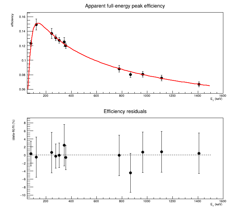
Eurica gamma 探测阵列由 12 个 Euroball Cluster 组成,每个 Cluster 含 7 个 HPGe 晶体;标定源距探测器约 22 cm。数据已对每个 Cluster 的 7 个晶体作 add-back,再合并 12 个 Cluster,用于考察阵列的整体性能。装置详情见 Installation and commissioning of EURICA – Euroball-RIKEN Cluster Array。
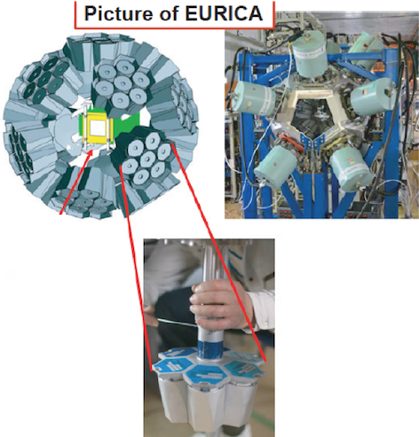
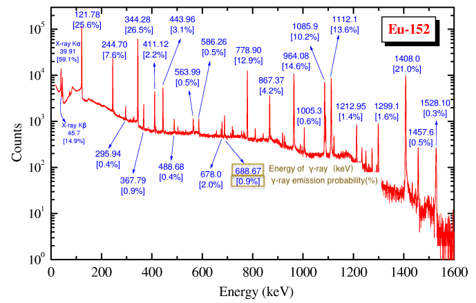
能谱由 $^{152}$Eu 与 $^{133}$Ba 标准源测得,测量开始于 2013 年 2 月 13 日,记录时长为 7442 s。两个源的参考日期均为 1998 年 1 月 1 日;参考活度分别为 $^{152}$Eu 40.9 kBq(5%)和 $^{133}$Ba 42.2 kBq(3%)。活度衰变修正采用 $T_{1/2}(^{152}\mathrm{Eu})=13.517$ y、$T_{1/2}(^{133}\mathrm{Ba})=3849.3$ d。
| Nuclide | Eγ (keV) | Pγ (%) |
|---|---|---|
| 133Ba | 80.9979 | 34.06 |
| 152Eu | 121.7817 | 28.41 |
| 152Eu | 244.6974 | 7.55 |
| 133Ba | 276.3989 | 7.164 |
| 133Ba | 302.8508 | 18.33 |
| 152Eu | 344.2785 | 26.59 |
| Nuclide | Eγ (keV) | Pγ (%) |
|---|---|---|
| 133Ba | 356.0129 | 62.05 |
| 152Eu | 778.9045 | 12.93 |
| 152Eu | 867.378 | 4.23 |
| 152Eu | 964.079 | 14.51 |
| 152Eu | 1112.076 | 13.67 |
| 152Eu | 1408.013 | 20.87 |
能量、$P_\gamma$ 和半衰期以推荐核数据为准,可查阅 DDEP/LNHB recommended decay data。$P_\gamma$ 是每次母核衰变发射该 gamma ray 的概率,不是源活度;较大的 $P_\gamma$ 有助于寻找强峰,但实测峰面积还受源活度和探测效率影响。
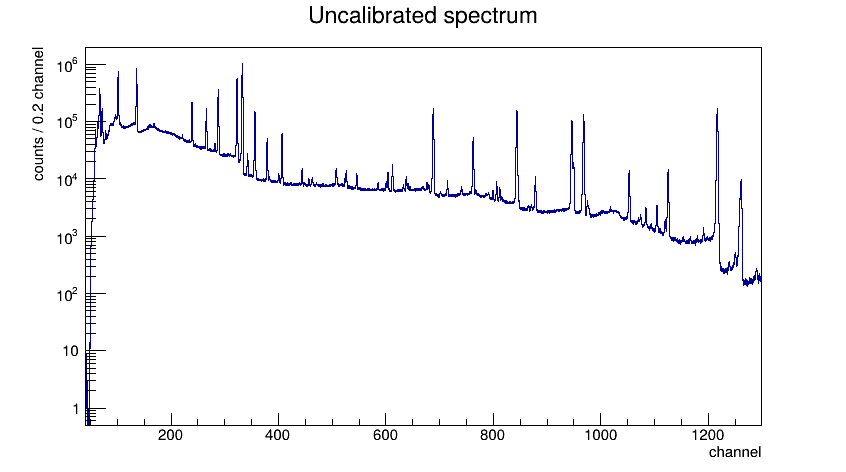
本作业使用 gamma.root 中的 TH1F h0。横轴尚未刻度,单位为 channel;每个 bin 宽 0.2 channel。
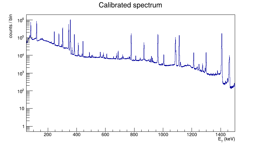
对照标准源参考能谱与上表,先辨认较强的谱线,再利用初步线性刻度寻找其余峰。
三项刻度使用同一组参考谱线,分别需要峰位、峰宽和净峰面积:
| 观测量 | 本作业采用的方法 | 用途 |
|---|---|---|
| 峰位 $\mu$ | Gaussian + 本底拟合 | 能量刻度 |
| $\sigma$、FWHM | 同一次拟合 | 分辨率刻度 |
| 孤立峰的 $N_{\rm net}$ | ROI summation 并扣除局部本底 | 效率刻度 |
| 重叠峰的各自面积 | fitting / deconvolution | 进阶分析 |
方法的依赖关系是
$$ \boxed{ \begin{aligned} \text{calibration-peak fits} &\rightarrow E(ch),\ \mathrm{FWHM}(E),\\ E_\gamma,\ E(ch),\ \mathrm{FWHM}(E) &\rightarrow \text{ROI center and width},\\ \text{ROI summation} &\rightarrow N_{\rm net}\rightarrow\varepsilon(E_\gamma). \end{aligned}} $$
先由峰拟合建立能量和分辨率刻度,再据此确定各参考线的 ROI。孤立峰的净面积直接由 ROI 计数扣除本底得到。
峰位、峰宽与局部本底
孤立、近似对称的 gamma 峰可先用 Gaussian 描述:
$$ s(x)=H\exp\!\left[-\frac{(x-\mu)^2}{2\sigma^2}\right]. $$
在较窄的峰区间内,平滑本底可先用直线近似:
$$ b(x)=b_0+b_1(x-x_0),\qquad f(x)=s(x)+b(x). $$
先在峰两侧选择不含峰信号的 sidebands,拟合直线,估计 $b_0$、$b_1$ 的初值;再在整个峰区间内同时拟合 Gaussian 和线性本底。此时本底参数也参与拟合。本例使用 binned Poisson likelihood 处理 histogram 计数。
拟合得到峰位、标准差和半高全宽:
$$ \mu,\qquad \sigma,\qquad \mathrm{FWHM}=2\sqrt{2\ln2}\,\sigma\simeq2.355\sigma. $$
除 fit status 外,还要检查 Pearson residual
$$ r_i=\frac{n_i-\nu_i}{\sqrt{\nu_i}}, $$
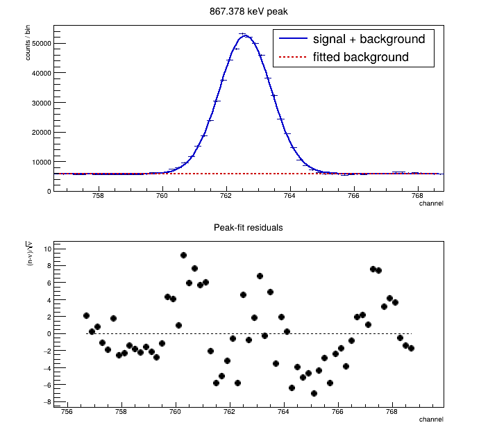
其中 $n_i$ 是观测计数,$\nu_i$ 是模型给出的期望计数。若 residual 在一段区域内持续偏正或偏负,应检查峰形和本底模型。
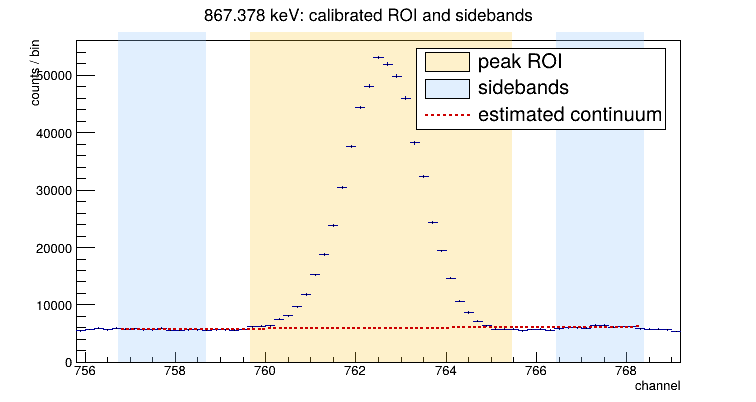
后面的代码以 867.378 keV 峰为例,使用 Gaussian + linear background,并在线性纵坐标下显示峰及两侧本底。
孤立峰的面积:ROI summation
完成刻度后,由参考线能量确定 ROI 中心,由 FWHM 确定窗口宽度:
$$ ch_0=E_{\rm cal}^{-1}(E_\gamma),\qquad W_{ch}=\frac{\mathrm{FWHM}(E_\gamma)}{ \left|dE_{\rm cal}/dch\right|_{ch_0}}. $$
本例使用以下 ROI 和 sidebands:
$$ \text{peak ROI}:\quad ch_0-1.5W_{ch}<ch<ch_0+1.5W_{ch}, $$
$$ \text{left sideband}:\quad ch_0-3W_{ch}<ch<ch_0-2W_{ch}, \qquad \text{right sideband}:\quad ch_0+2W_{ch}<ch<ch_0+3W_{ch}. $$
窗口宽度可根据谱形调整,sidebands 应避开邻峰和明显变化的本底。
设 peak ROI 的 gross counts 为 $G$,左右 sideband 的总计数分别为 $L$、$R$,包含的 bin 数分别为 $m_L$、$m_R$,peak ROI 含 $n$ 个 bins。对关于 peak 对称的窗口,linear continuum 在 peak ROI 下的计数估计为
$$ B=\frac{n}{2}\left(\frac{L}{m_L}+\frac{R}{m_R}\right), $$
因此
$$ \boxed{N_{\rm net}=G-B.} $$
若三个区域互不重叠,且 bin counts 服从 Poisson statistics,则
$$ \boxed{ u^2(N_{\rm net})= G+\left(\frac{n}{2m_L}\right)^2L +\left(\frac{n}{2m_R}\right)^2R. } $$
第一项来自 peak ROI 的计数涨落,后两项来自用 sidebands 估计本底的计数涨落。
本作业对孤立峰采用 ROI summation。重叠峰的各自面积不能用单个 ROI 区分,需要多峰拟合。
能量、分辨率与效率刻度
能量刻度
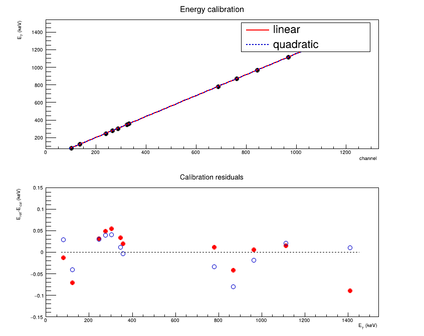
用各参考线的 centroid $ch_i$ 与已知能量 $E_i$ 拟合
$$E(ch)=a_0+a_1ch.$$
先由两个相隔较远、指认可靠的 peak 建立粗略线性关系,再据此定位其余参考线。最终用 calibration residual
$$\Delta E_i=E_{i,\mathrm{ref}}-E_{\mathrm{cal}}(ch_i)$$
检查刻度;只有 residual 呈现系统曲率时才考虑加入 $a_2ch^2$。把刻度应用到完整 histogram 后,变换前后的总计数应保持一致。
能量分辨率
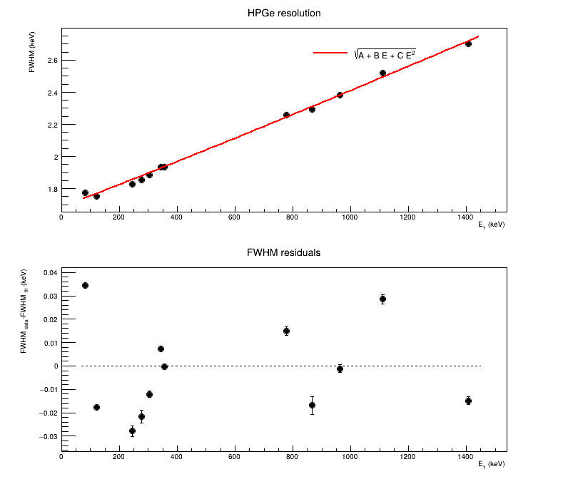
由能量刻度的局部斜率把 channel 上的 width 换算为
$$ FWHM(E)=2\sqrt{2\ln2}\left|\frac{dE}{dch}\right|\sigma_{ch} \approx2.355\left|\frac{dE}{dch}\right|\sigma_{ch}. $$
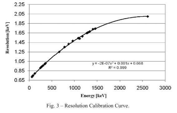
Gaussian peak 满足 $FWHM=2.355\sigma_E$,因此 FWHM 与 $\sigma_E$ 具有相同的能量依赖。如果载流子数目的统计涨落占主导,则 $\sigma_E^2\propto E$,从而 $\sigma_E$ 和 FWHM 均正比于 $\sqrt{E}$。
实际 HPGe 还包含电子学噪声和电荷收集等贡献,这些近似独立的贡献在方差层面相加,因此常用
$$FWHM(E)=\sqrt{A+BE+CE^2}$$
其中 $A$、$BE$ 和 $CE^2$ 分别概括电子学噪声、载流子统计和随能量增长的电荷收集等贡献。当 $BE$ 项占主导时,公式回到 $FWHM\propto\sqrt{E}$;完整曲线在有限能区内可能外观上接近直线,但这不是 FWHM 的一般线性规律。得到的 $FWHM(E)$ 既描述探测器分辨率,也可作为全谱选取 peak ROI 与 sidebands 的自然尺度。
Full-energy peak efficiency
把参考活度 $A_0$ 从日期 $t_0$ 修正到测量日期 $t$:
$$ A(t)=A_0\,2^{-(t-t_0)/T_{1/2}}. $$
对每条已知参考线,由最终刻度确定 ROI 并扣除局域本底,再用 net peak area 计算
$$ \boxed{ \varepsilon(E_\gamma)= \frac{N_{\rm net}}{A(t)P_\gamma t_{\rm live}}. } $$
若输入量相互独立,且 live time 的误差可忽略,单个效率点的相对误差为
$$ \left(\frac{u_\varepsilon}{\varepsilon}\right)^2= \left(\frac{u_N}{N_{\rm net}}\right)^2+ \left(\frac{u_A}{A(t)}\right)^2+ \left(\frac{u_P}{P_\gamma}\right)^2. $$
同一标准源的活度误差会同时移动该源的全部 efficiency 点,是相关的 normalization uncertainty,不是彼此独立的 point-to-point fluctuation。
若尚未修正 dead time、true-coincidence summing、源几何、衰减与自吸收,这里得到的是该测量设置下的 apparent full-energy peak efficiency。实例暂把题目给出的 7442 s 作为 $t_{\rm live}$;若采集记录区分 real time 与 live time,应使用 live time。
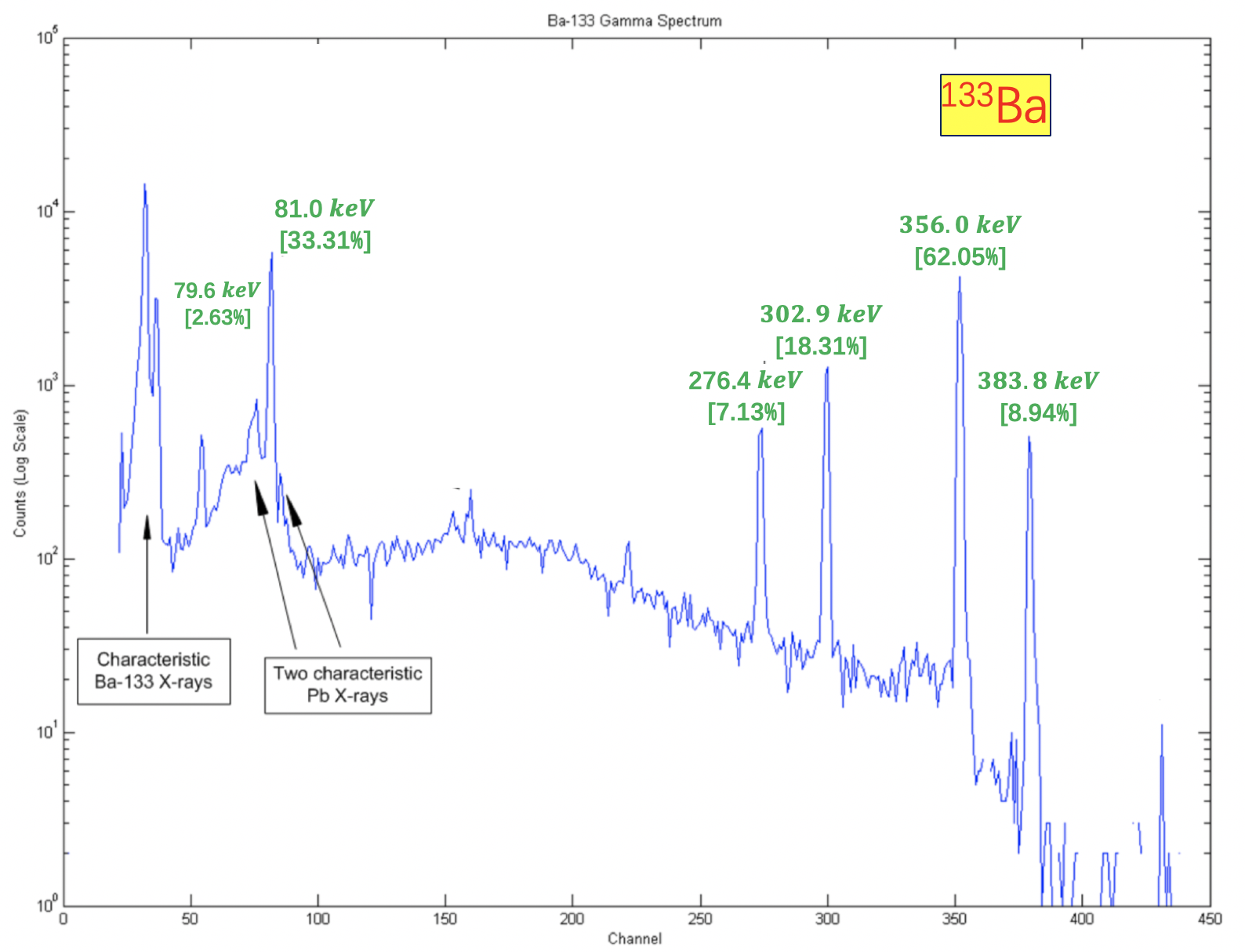
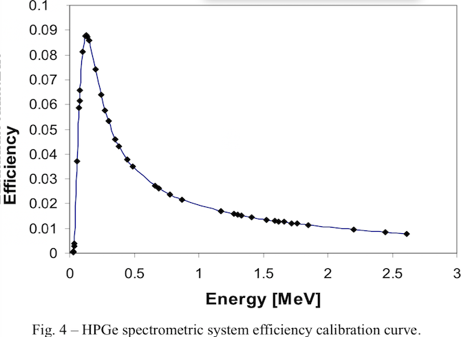
HPGe 的 efficiency 在低能端会因端帽、死层和源封装材料的吸收而下降,在中间能区达到最大值后再随能量升高而下降。令
$$u=\ln\!\left(\frac{E}{100\ \mathrm{keV}}\right),$$
本作业采用经验函数
$$ \varepsilon(E)=\exp\!\left[ p_0+p_1u+p_2u^2-p_3\left(\frac{100\ \mathrm{keV}}{E}\right)^3 \right],\qquad p_3\ge0. $$
效率图的横、纵坐标均采用线性刻度,并检查相对 residual。本数据最低参考能量为 81 keV,更低能区没有刻度点约束。
进阶:复杂本底与重叠峰
linear background 只是在窄区间内对 smooth continuum 的一阶近似。实际 gamma spectrum 还可能包含 Compton continuum 或 edge、邻近 peak、低能 tail 和电子学响应。
- 若 peak 前后的 background level 存在明显 step,可在 linear term 上加入 $\frac{S}{2}\operatorname{erfc}[(x-\mu)/(\sqrt2\sigma)]$;只有 residual 明显改善时才需要增加参数。本数据的 1408 keV peak 试算没有得到实质改善,因此主分析仍采用 linear background。
- 非 Gaussian peak 可在响应函数中加入 low-energy tail。
ORTEC GammaVision 用户手册以 straight-line background 作为基本 ROI/singlet 处理,并在谱形需要时提供 stepped 或 parabolic background。肖石良等(2024)对更复杂的在线 gamma spectrum 分别加入低能 tail、erfc step、polynomial background 和 Compton-edge response;单个 erfc 项不能解释所有本底结构。
Multiplet
多个峰重叠时,可把整个区域的计数密度写为
$$ f(x)=b(x)+\sum_k N_k p_k(x),\qquad \int p_k(x)\,dx=1, $$
对每个 bin 积分得到期望计数后进行拟合,此时 $N_k$ 表示第 $k$ 个峰的面积。$C$ 是拟合返回的参数 covariance matrix,单个面积误差为 $u(N_k)=\sqrt{C_{kk}}$,即该面积参数的拟合误差;计算总面积或强度比时还要保留非对角项 $C_{ij}$。若两个面积高度相关,说明各峰强度不易分别确定。已知能量和 $\mathrm{FWHM}(E)$ 可用于约束峰位和峰宽。
给定能量处的效率曲线误差
给定能量处的效率曲线误差由拟合参数的 covariance 传播得到。计算方法见加权拟合与拟合结果的误差传播。本例曲线拟合的权重未计入活度的相关误差,因此该误差还不包含活度归一化和模型选择的影响。
作业要求
- 对照标准源谱线,在完整能谱中指认参考峰。用 Gaussian + linear background 拟合孤立峰,提取峰位、$\sigma$ 和 FWHM,并检查 residual。
- 用峰位与已知能量建立线性能量刻度;若残差有系统曲率,再比较二次函数。将选定刻度应用到完整能谱,检查总计数是否保持不变。
- 将各峰的宽度换算为 keV,绘制 FWHM–$E_\gamma$ 曲线,用 $\sqrt{A+BE+CE^2}$ 拟合并检查 residual。
- 由能量与分辨率刻度确定各参考线的 ROI,扣除本底得到净峰面积及其计数误差。修正标准源活度后,计算 apparent full-energy peak efficiency,绘制效率曲线与相对 residual;横纵坐标均使用线性刻度。
进度对应第 3 章。
实例代码
以下用 867.378 keV 峰分步说明峰位、峰宽和净面积的提取。先拟合峰位与峰宽;完成能量和分辨率刻度后,再用刻度曲线确定 ROI 并求净面积。批量处理参考线的代码见完整实例。
读取并查看能谱
先打开文件并取得 h0。%jsroot on(PyROOT)和 //%jsroot on(ROOT C++)开启 notebook 中的交互式图形。完整谱使用对数纵坐标,以便同时观察强峰与弱峰。
import math
import ROOT

%jsroot on
ROOT.gStyle.SetOptStat(0)

# TFile.Open 打开 ROOT 文件;Get 取得其中名为 h0 的 histogram。
input_file = ROOT.TFile.Open("gamma.root", "READ")
h0 = input_file.Get("h0")

c_spectrum = ROOT.TCanvas("c_spectrum_py", "h0", 850, 480)
c_spectrum.SetLogy()
h0.SetTitle("^{152}Eu + ^{133}Ba spectrum;channel;counts / bin")
h0.GetXaxis().SetRangeUser(40, 1300)
h0.SetMinimum(0.5)
h0.Draw("hist")
c_spectrum.Draw()
c_spectrum.SaveAs("standard_source_spectrum.png")
//%jsroot on
#include "TCanvas.h"
#include "TFile.h"
#include "TF1.h"
#include "TFitResultPtr.h"
#include "TGraph.h"
#include "TGraphErrors.h"
#include "TH1.h"
#include "TLine.h"
#include "TStyle.h"
#include <algorithm>
#include <cmath>
#include <iomanip>
#include <iostream>

gStyle->SetOptStat(0);

// TFile::Open 打开 ROOT 文件;Get 取得其中名为 h0 的 histogram。
auto inputFile = TFile::Open("gamma.root", "READ");
auto h0 = dynamic_cast<TH1*>(inputFile->Get("h0"));

auto cSpectrum = new TCanvas("cSpectrum", "h0", 850, 480);
cSpectrum->SetLogy();
h0->SetTitle("^{152}Eu + ^{133}Ba spectrum;channel;counts / bin");
h0->GetXaxis()->SetRangeUser(40, 1300);
h0->SetMinimum(0.5);
h0->Draw("hist");
cSpectrum->Draw();
cSpectrum->SaveAs("standard_source_spectrum.png");
第一阶段:拟合 867.378 keV 峰
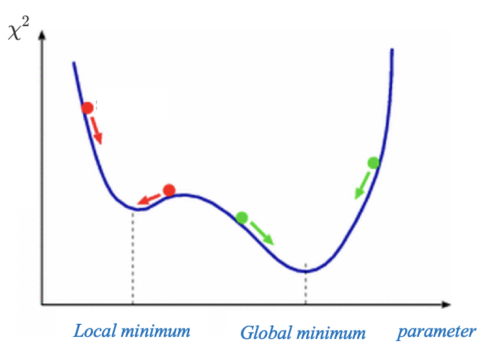
多参数 fit 从给定初值开始搜索。初值偏离数据太远时,minimizer 可能进入错误的 local minimum 或不能稳定收敛。可以先从谱图估计参数量级,再让拟合确定参数。下图说明不同初值可能影响搜索路径。
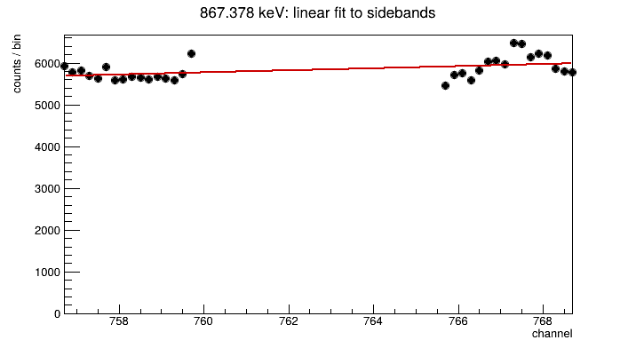
先查看峰及两侧本底。左右 sidebands 的直线拟合给出 $b_0$ 与 slope 的初值;峰顶计数减去本底可估计峰高 $H$,峰的位置和宽度可估计 $\mu$、$\sigma$。用 parameter limits 限定峰高、宽度等参数的物理范围。
本例会用到 SetParameter 设置初值、SetParLimits 设置允许范围、GetParameter / GetParError 读取结果,以及 Integral 计算每个 bin 的模型期望。
fit option LIRSQN 中,L 选择 binned Poisson likelihood,I 使用函数在每个 bin 内的平均值,即积分除以 bin 宽,R 使用 TF1 的局部范围,S 返回参数误差、covariance 等完整拟合结果,Q 关闭详细输出,N 不自动把函数附着到 histogram 或绘图。
先拟合 sidebands
先排除峰所在的区间,用左右 sidebands 拟合直线,给下一步的峰与本底联合拟合提供初值。
xmin867, xmax867 = 756.7, 768.7
sideband_graph867 = ROOT.TGraphErrors()
point = 0
for bin_number in range(h0.FindBin(xmin867), h0.FindBin(xmax867) + 1):
    x = h0.GetBinCenter(bin_number)
    if 759.7 < x < 765.7:       # exclude the visible peak
        continue
    count = h0.GetBinContent(bin_number)
    sideband_graph867.SetPoint(point, x, count)
    sideband_graph867.SetPointError(point, 0.0, math.sqrt(max(count, 1.0)))
    point += 1

background_seed867 = ROOT.TF1(
    "background_seed867_py", "[0]+[1]*(x-762.7)", xmin867, xmax867
)
background_seed867.SetParameters(5.8e3, 0.0)
sideband_graph867.Fit(background_seed867, "RQN")
double xmin867 = 756.7;
double xmax867 = 768.7;
auto sidebandGraph867 = new TGraphErrors();
int sidebandPoint867 = 0;
for (int bin = h0->FindBin(xmin867); bin <= h0->FindBin(xmax867); ++bin) {
    double x = h0->GetBinCenter(bin);
    if (x > 759.7 && x < 765.7) continue;  // exclude the visible peak
    double count = h0->GetBinContent(bin);
    sidebandGraph867->SetPoint(sidebandPoint867, x, count);
    sidebandGraph867->SetPointError(
        sidebandPoint867, 0.0, std::sqrt(std::max(count, 1.0)));
    ++sidebandPoint867;
}

auto backgroundSeed867 = new TF1(
    "backgroundSeed867", "[0]+[1]*(x-762.7)", xmin867, xmax867);
backgroundSeed867->SetParameters(5.8e3, 0.0);
sidebandGraph867->Fit(backgroundSeed867, "RQN");
同时拟合峰与本底
用 sideband fit 初始化本底,再在完整区间内同时拟合 Gaussian 与 linear background。此时 b0 和 slope 没有固定,会与 peak parameters 一起由数据确定。
model867 = "gaus(0)+[3]+[4]*(x-762.7)"
f867 = ROOT.TF1("f867_py", model867, xmin867, xmax867)
f867.SetParNames("height", "mean", "sigma", "b0", "slope")
f867.SetParameter(0, 4.5e4)                                # peak height
f867.SetParameter(1, 762.7)                               # centroid
f867.SetParameter(2, 0.8)                                 # sigma
f867.SetParameter(3, background_seed867.GetParameter(0))  # b0 from sidebands
f867.SetParameter(4, background_seed867.GetParameter(1))  # slope from sidebands
f867.SetParLimits(0, 0.0, 1.0e7)
f867.SetParLimits(1, 760.5, 765.0)
f867.SetParLimits(2, 0.2, 3.0)

result867 = h0.Fit(f867, "LIRSQN")

mean867 = f867.GetParameter(1)
sigma867 = abs(f867.GetParameter(2))
fwhm867 = 2.0 * math.sqrt(2.0 * math.log(2.0)) * sigma867

print(f"centroid = {mean867:.4f} +/- {f867.GetParError(1):.4f} channel")
print(f"sigma    = {sigma867:.4f} +/- {f867.GetParError(2):.4f} channel")
print(f"FWHM     = {fwhm867:.4f} channel")
print(f"fit status = {int(result867)}")
auto f867 = new TF1(
    "f867", "gaus(0)+[3]+[4]*(x-762.7)", xmin867, xmax867);
f867->SetParNames("height", "mean", "sigma", "b0", "slope");
f867->SetParameter(0, 4.5e4);                              // peak height
f867->SetParameter(1, 762.7);                             // centroid
f867->SetParameter(2, 0.8);                               // sigma
f867->SetParameter(3, backgroundSeed867->GetParameter(0)); // b0 from sidebands
f867->SetParameter(4, backgroundSeed867->GetParameter(1)); // slope from sidebands
f867->SetParLimits(0, 0.0, 1.0e7);
f867->SetParLimits(1, 760.5, 765.0);
f867->SetParLimits(2, 0.2, 3.0);

TFitResultPtr result867 = h0->Fit(f867, "LIRSQN");

double mean867 = f867->GetParameter(1);
double sigma867 = std::abs(f867->GetParameter(2));
double fwhm867 = 2.0 * std::sqrt(2.0 * std::log(2.0)) * sigma867;

std::cout << std::fixed << std::setprecision(4)
          << "centroid = " << mean867 << " +/- " << f867->GetParError(1)
          << " channel\nsigma    = " << sigma867 << " +/- "
          << f867->GetParError(2) << " channel\nFWHM     = " << fwhm867
          << " channel\nfit status = " << static_cast<int>(result867) << std::endl;
centroid = 762.6016 +/- 0.0015 channel
sigma    = 0.8180 +/- 0.0014 channel
FWHM     = 1.9263 channel
fit status = 0
Fit 与 residual 图
用 TF1::Integral 对每个 bin 积分后除以 bin 宽,得到与 fit option I 一致的期望计数。上图显示数据、总模型和拟合本底,下图显示 Pearson residual。
residual867 = ROOT.TGraph()
for point, bin_number in enumerate(
    range(h0.FindBin(xmin867), h0.FindBin(xmax867) + 1)
):
    low = h0.GetBinLowEdge(bin_number)
    width = h0.GetBinWidth(bin_number)
    expected = f867.Integral(low, low + width) / width
    observed = h0.GetBinContent(bin_number)
    residual867.SetPoint(
        point, h0.GetBinCenter(bin_number),
        (observed - expected) / math.sqrt(expected)
    )
auto residual867 = new TGraph();
int point867 = 0;
for (int bin = h0->FindBin(xmin867); bin <= h0->FindBin(xmax867); ++bin) {
    double low = h0->GetBinLowEdge(bin);
    double width = h0->GetBinWidth(bin);
    double expected = f867->Integral(low, low + width) / width;
    double observed = h0->GetBinContent(bin);
    residual867->SetPoint(
        point867++, h0->GetBinCenter(bin),
        (observed - expected) / std::sqrt(expected));
}
第二阶段:由全局刻度确定 ROI 并求面积
GetX 用已知 $E_\gamma$ 反求 channel;Derivative 把 keV 中的 FWHM 换回 channel。为使示例可独立运行,下面暂用给定参数构造两条全局刻度曲线;完成作业时应换成自己得到的 calibration 和 width_model。
calibration_for_roi = ROOT.TF1("calibration_for_roi_py", "[0]+[1]*x", 40.0, 1300.0)
calibration_for_roi.SetParameters(-39.924169, 1.189801088)
width_model_for_roi = ROOT.TF1(
    "width_model_for_roi_py",
    "sqrt([0]+[1]*x+[2]*x*x)", 70.0, 1450.0
)
width_model_for_roi.SetParameters(2.83349, 0.002312, 6.5270e-7)

energy867 = 867.378
center867 = calibration_for_roi.GetX(energy867, 40.0, 1300.0)
kev_per_channel867 = abs(calibration_for_roi.Derivative(center867))
fwhm867_for_area = width_model_for_roi.Eval(energy867) / kev_per_channel867

left_low867 = center867 - 3.0*fwhm867_for_area
left_high867 = center867 - 2.0*fwhm867_for_area
roi_low867 = center867 - 1.5*fwhm867_for_area
roi_high867 = center867 + 1.5*fwhm867_for_area
right_low867 = center867 + 2.0*fwhm867_for_area
right_high867 = center867 + 3.0*fwhm867_for_area
auto calibrationForRoi = new TF1("calibrationForRoi", "[0]+[1]*x", 40.0, 1300.0);
calibrationForRoi->SetParameters(-39.924169, 1.189801088);
auto widthModelForRoi = new TF1(
    "widthModelForRoi",
    "sqrt([0]+[1]*x+[2]*x*x)", 70.0, 1450.0);
widthModelForRoi->SetParameters(2.83349, 0.002312, 6.5270e-7);

double energy867 = 867.378;
double center867 = calibrationForRoi->GetX(energy867, 40.0, 1300.0);
double kevPerChannel867 = std::abs(calibrationForRoi->Derivative(center867));
double fwhm867ForArea = widthModelForRoi->Eval(energy867) / kevPerChannel867;

double leftLow867 = center867 - 3.0*fwhm867ForArea;
double leftHigh867 = center867 - 2.0*fwhm867ForArea;
double roiLow867 = center867 - 1.5*fwhm867ForArea;
double roiHigh867 = center867 + 1.5*fwhm867ForArea;
double rightLow867 = center867 + 2.0*fwhm867ForArea;
double rightHigh867 = center867 + 3.0*fwhm867ForArea;
积分并扣除本底
FindBin 把窗口边界换成 bin number;TH1::Integral 累加选中 bins 的计数,与前面 TF1::Integral 的函数积分不同。边界移动半个 bin,用于按 bin center 选择窗口内的 bins。
half_bin = 0.5*h0.GetBinWidth(1)
l1 = h0.FindBin(left_low867 + half_bin)
l2 = h0.FindBin(left_high867 - half_bin)
p1 = h0.FindBin(roi_low867 + half_bin)
p2 = h0.FindBin(roi_high867 - half_bin)
r1 = h0.FindBin(right_low867 + half_bin)
r2 = h0.FindBin(right_high867 - half_bin)

left867 = h0.Integral(l1, l2)
gross867 = h0.Integral(p1, p2)
right867 = h0.Integral(r1, r2)
m_left867 = l2 - l1 + 1
n_roi867 = p2 - p1 + 1
m_right867 = r2 - r1 + 1

weight_left867 = 0.5*n_roi867/m_left867
weight_right867 = 0.5*n_roi867/m_right867
background_count867 = weight_left867*left867 + weight_right867*right867
net867 = gross867 - background_count867
net_error867 = math.sqrt(
    gross867 + weight_left867**2*left867 + weight_right867**2*right867
)

print(f"G = {gross867:.0f}")
print(f"B = {background_count867:.1f}")
print(f"N_net = {net867:.1f} +/- {net_error867:.1f}")
double halfBin = 0.5*h0->GetBinWidth(1);
int l1 = h0->FindBin(leftLow867 + halfBin);
int l2 = h0->FindBin(leftHigh867 - halfBin);
int p1 = h0->FindBin(roiLow867 + halfBin);
int p2 = h0->FindBin(roiHigh867 - halfBin);
int r1 = h0->FindBin(rightLow867 + halfBin);
int r2 = h0->FindBin(rightHigh867 - halfBin);

double left867 = h0->Integral(l1, l2);
double gross867 = h0->Integral(p1, p2);
double right867 = h0->Integral(r1, r2);
int mLeft867 = l2 - l1 + 1;
int nRoi867 = p2 - p1 + 1;
int mRight867 = r2 - r1 + 1;

double weightLeft867 = 0.5*nRoi867/mLeft867;
double weightRight867 = 0.5*nRoi867/mRight867;
double backgroundCount867 = weightLeft867*left867 + weightRight867*right867;
double net867 = gross867 - backgroundCount867;
double netError867 = std::sqrt(
    gross867 + weightLeft867*weightLeft867*left867
    + weightRight867*weightRight867*right867);

std::cout << std::fixed << std::setprecision(0)
          << "G = " << gross867 << "\n"
          << std::setprecision(1) << "B = " << backgroundCount867 << "\n"
          << "N_net = " << net867 << " +/- " << netError867 << std::endl;
G = 648546
B = 171471.8
N_net = 477074.2 +/- 954.2