Relativistic Kinetics

Mechanics in special relativity

This section explores the Lorentz transformation, relativistic energy and momentum, natural units, and the powerful formalism of 4-vectors, providing a cohesive framework for analyzing physical systems moving at relativistic speeds.

Lorentz transformation

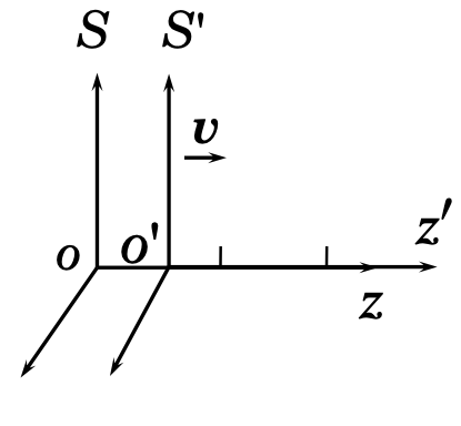
In special relativity, space and time coordinates depend on the observer’s inertial frame of reference. Consider two inertial frames: one at rest (S) and another moving at velocity ( v ) along the +z-axis relative to it (S'). The Lorentz Transformation (LT) relates the coordinates (ct, x, y, z) in the rest frame to (ct', x', y', z') in the moving frame as follows:

$$ \begin{align} x' &= x & x &= x' \\ y' &= y & y &= y' \\ z' &= \gamma (z - \beta ct) & z &= \gamma (z' + \beta ct) \\ ct' &= \gamma (ct - \beta z) & ct &= \gamma (ct' + \beta z) \end{align} $$

where:

• $β=v/c$, with ( c ) as the speed of light,
• $γ=1/1−β^2$, the Lorentz factor.

Key properties of the LT include: Invariance of the spacetime interval:

• The quantity $s^2 = (ct)^2 - x^2 - y^2 - z^2$ remains constant across all inertial frames, reflecting the fundamental structure of spacetime in special relativity.

• Transverse lengths unchanged: Coordinates perpendicular to the direction of motion ( x ) and ( y ) are unaffected.

• Length contraction: Along the direction of motion, the length of an object in the moving frame ($\Delta z'$) relates to its proper length (at rest, $\Delta z$) as $\Delta z' = \Delta z / \gamma$, meaning a moving object appears shorter.

• Time dilation: The measured time interval of a moving clock is related to the elapsed time at rest (primed frame) by Δt‘ = γ Δt , i.e. time dilation. We call a time interval for an object at rest the “proper time” τ. Thus t‘ = γτ and t’ ≥ τ . The proper time concept is useful when comparing the lifetime of a particle in its rest frame and in the frame in which it is moving.

Relativistic energy and momentum

Relativistic mechanics extends classical definitions of momentum and energy to account for high velocities. For a particle with velocity $v$:

• Momentum: $p = \gamma m v$, where $m$ is the rest mass.

• Total energy: $E = \gamma m c^2$, encompassing both rest energy $m c^2$ and kinetic energy.

In the same coordinate frames as the LT, the energy-momentum transformations mirror the spacetime ones:

$$ \begin{align} &p'_x = p_x &p_x =& p'_x \\ &p'_y = p_y &p_y = &p'_y\\ &p'_z = γ (p_z − βE/c) &p_z =& γ (p'_z + βE/c)\\ &E'/c = γ (E/c − βp_z) &E/c =& γ (E'/c + βp_z) \end{align} $$

Key relationships include:

• Invariant mass: The quantity $(E/c)^2 - p_x^2 - p_y^2 - p_z^2 = m^2 c^2$ is preserved under LT, defining the rest mass $m$ as an invariant property.

• Momentum magnitude: $p = \gamma \beta m c$.

• Kinetic energy: $E_K = E - m c^2 = (\gamma - 1) m c^2$.

• Energy-momentum relation: $E^2 = (p c)^2 + (m c^2)^2$, linking energy, momentum, and rest mass.

• Mentum-Kinetic energy relation: $(pc)^2 = E_k^2+2mc^2E_K$

For massless particles (e.g., photons), $m = 0$, so $E = p c$, and their speed is always $c$. For highly relativistic particles ($E \gg m c^2$), $E \approx p c$ and $v \approx c$, resembling massless behavior.

Natural units

In relativistic kinematics, natural units simplify calculations by setting $c = 1$, expressing energy, momentum, and mass in GeV .

Key relationships in natural units:

• Invariant mass: $E^2 - p_x^2 - p_y^2 - p_z^2 = m^2 $

• Momentum magnitude: $p = \gamma \beta m$.

• Kinetic energy: $E_K = E - m = (\gamma - 1) m$.

• Energy-momentum relation: $E^2 = p^2 + m^2$.

• Kinetic Energy-momentum relation: $p^2 = E_k^2+2mE_K$

Published literature often uses GeV/$c^2$ for mass and GeV/$c$ for momentum to retain dimensional clarity in SI units, but in natural units, these factors of $c$ are omitted. Conversions to SI units require GeV = 1.602 $\times 10^{-10} \, J$ and $c = 3 \times 10^8 \, m/s$ .

Example

Consider a $K_s$(K-short) meson with rest mass $m_{Ks} = 0.4977$ GeV moving along the +z-axis at $v = 0.95c$ in natural units:

• $γ_{Ks} =1/\sqrt{1−0.95^2} = 3.202563$

• $E_{Ks} =γ_{Ks} m_{Ks}=3.202563×0.4977 = 1.593916 \text{ GeV}$

• $p_{z_{Ks}} =γ_{Ks}\beta_{Ks}m_{Ks} =3.202563×0.4977×0.95 = 1.514220 \text{ GeV}$, with $p_x=p_y=0$

Check invariance: $m = \sqrt{E^2 - p^2} = \sqrt{(1.593916)^2 - (1.514220)^2} = 0.4977$ GeV , matching the rest mass. In SI units, mass is $0.4977$ GeV/$c^2$, momentum is $1.514220$ GeV/$c$, convertible using standard constants. This example highlights the $K_s$ meson’s relativistic nature, with $E \approx 3m c^2$, approaching massless-like behavior $E \approx p$.

Vectors and Lorentz Transformations

The 4-vector formalism unifies spacetime and energy-momentum, streamlining relativistic analysis.

Definition of 4-Vectors

A 4-vector combines a time like component with a spatial 3-vector:

• Spacetime 4-vector: $X = (ct, \vec{x}) = (ct, x, y, z)$,

• Energy-momentum 4-vector: $P = (E/c, \vec{p}) = (E/c, p_x, p_y, p_z)$

.

For any 4-vector $A = (A_0, \vec{A})$, the 3-vector magnitude is $|\vec{A}|^2 = A_1^2 + A_2^2 + A_3^2$.

Lorentz Transformation of 4-Vectors

The LT applies to 4-vectors, preserving their inner product:

• Inner product: $A \cdot B = A_0 B_0 - \vec{A} \cdot \vec{B} = A_0 B_0 - A_1 B_1 - A_2 B_2 - A_3 B_3$,

• Norm: $A^2 = A \cdot A = A_0^2 - |\vec{A}|^2$

, invariant across frames.

For P:

• $P \cdot P = (E/c)^2 - |\vec{p}|^2 = m^2 c^2$, $P^2 = E^2 - p^2 = m^2$ in natural units, .

In the rest frame: $P = (m, 0, 0, 0)$, so $P^2 = m^2$, consistent in all frames.

Linear combinations of 4-vectors (e.g., $C = aA + bB$) are also 4-vectors, making this a versatile tool.

Multi-Particle Systems

For a system of particles, the total 4-momentum $P_{\text{total}} = \sum P_i$ has an invariant norm: $$ P_{\text{total}}^2 = \left( \sum E_i \right)^2 - \left| \sum \vec{p}_i \right|^2 $$ useful in decay or collision processes.

Conservation in Reactions

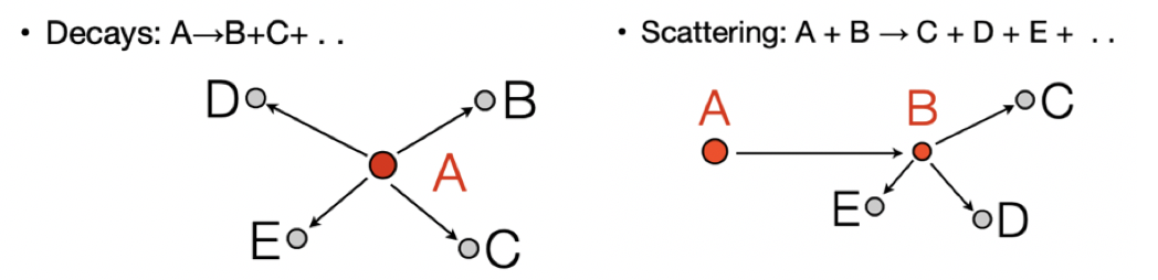
In a decay $P \to P_1 + P_2 + P_3$ or scattering $P_1 + P_2 \to P_3 + P_4$, 4-momentum conservation $P_{\text{initial}} = P_{\text{final}}$ automatically enforces both energy and momentum conservation, simplifying analysis.

Physics Vectors

In physics, vectors are essential for describing quantities with magnitude and direction, such as position, displacement, momentum, and energy. This section introduces vector classes in 2D, 3D, and 4D (Lorentz vectors), focusing on their representations and transformations, with practical implementations in the CERN ROOT framework. Building on the relativistic mechanics discussed earlier, we’ll connect these concepts to the 4-vector formalism and Lorentz transformations used in special relativity.

Vector Classes and Representations

Vectors can be defined in various dimensions and coordinate systems, depending on the physical context. The ROOT library, widely used in high-energy physics, provides modern classes for handling these vectors with double-precision arithmetic, replacing legacy types like TVector3 and TLorentzVector.

Tutorial: TVector3, TLorentzVector

This tutorial explores the usage of the legacy TVector3 and TLorentzVector classes alongside their modern counterparts in the CERN ROOT framework. It focuses on their representations, properties, transformations, and applications in physics, particularly in 3D spatial vectors and 4D Lorentz vectors for relativistic calculations. This builds on the vector concepts introduced earlier, emphasizing their practical utility in high-energy physics. A key distinction between legacy and modern classes lies in precision, flexibility, and compatibility, with modern classes offering improved double-precision arithmetic and support for diverse coordinate systems, while legacy classes remain simpler and more compatible with older ROOT codebases.

• Modern ROOT Physics Vector Classes

https://root.cern.ch/doc/master/group__GenVector.html

3D Vectors: TVector3

https://root.cern.ch/doc/master/classTVector3.html

The TVector3 class is a legacy ROOT type for representing 3D displacement vectors, typically in Cartesian coordinates $(x, y, z)$. It is commonly applied to spatial quantities like position, displacement, or momentum components in particle physics.

Representations

• Cartesian: Defined as $(x, y, z)$, accessible via methods like X(), Y(), and Z() (or Px(), Py(), Pz() for momentum-like vectors).
• Spherical: Converted internally using magnitude (Mag()), polar angle (Theta()), and azimuthal angle (Phi()).

Properties

• Magnitude: Computed as $\sqrt{x^2 + y^2 + z^2}$.
• Direction: Expressed through $\theta$ (polar angle) and $\phi$ (azimuthal angle).
• These vectors are foundational for describing particle trajectories or detector coordinates.

Member Functions

• Set values with:

  • SetX(x), SetY(y), SetZ(z): Individual components.

  • SetXYZ(x, y, z): Full Cartesian vector.

  • SetMag(Double_t)

  • SetMagThetaPhi(mag, theta, phi): Setter with mag, theta, phi.

  • SetPhi (Double_t): Set phi keeping mag and theta constant (BaBar).

  • SetTheta (Double_t): Set theta keeping mag and phi constant (BaBar).

  • TVector3 Unit () const: Return unit vector parallel to this.

  • TVector3 &Transform (const TRotation &): Transform this vector with a TRotation.

Transformations

• Rotation: RotateX(angle), RotateY(angle), RotateZ(angle) rotate the vector around the respective axes by a specified angle (in radians).
• General rotation: Rotate(angle, axis) rotates the vector around a custom TVector3 axis by the given angle.

4D Lorentz Vectors: TLorentzVector

https://root.cern.ch/doc/master/classTLorentzVector.html

The TLorentzVector class represents 4-vectors in special relativity, combining spatial and temporal (or momentum and energy) components, typically in the form $(p_x, p_y, p_z, E)$ in natural units ($c = 1$). It is straightforward but lacks the versatility of modern alternatives.

Representations

• Cartesian: Defined as $(p_x, p_y, p_z, E)$, representing the energy-momentum 4-vector $P = (E, \vec{p})$.

Properties

• 3D vector: Rho(),Theta(),Phi(),Vect()
• Momentum components: Px(), Py(), Pz().
• Energy: E().
• Invariant mass: M(), computed as $\sqrt{E^2 - p^2}$.
• Transverse momentum: Pt(), given by $\sqrt{p_x^2 + p_y^2}$.
• Pseudorapidity: Eta(), and azimuthal angle: Phi().

Member Functions

• Set values with:
  • SetPx(px), SetPy(py), SetPz(pz), SetE(e): Individual components.
  • SetPxPyPzE(px, py, pz, e): Full energy-momentum vector.
  • SetXYZM(px, py, pz, M): Full momentum-mass vector.
  • SetVect(TVector3 v):
  • SetRho(rho):
  • SetTheta(theta):
  • SetPhi(phi):

Transformations

• Lorentz boost: Boost(boostVector) applies a Lorentz transformation using a TVector3 boost velocity vector.
• Rotation: RotateX(angle), RotateY(angle), RotateZ(angle) rotate the spatial components around the respective axes.

Example: 4-vector for a K_s meson

A K_s meson’s 4-vector can be defined using TLorentzVector with $(p_x, p_y, p_z, E)$. Properties like mass, transverse momentum, and $\beta,\gamma$ can be extracted.

// Example using the TLorentzVector class in ROOT
#include <iostream>
#include "TLorentzVector.h"  // 4-vector class from ROOT

// Define a 4-vector for a K_s meson 
TLorentzVector ks(0.0, 0.0, 1.5142202, 1.5939162); // (px, py, pz, E)

// Print momentum and energy components
std::cout << "K_s Meson 4-Vector (TLorentzVector):\n";
std::cout << Form("  Px = %.3f GeV, Py = %.3f GeV, Pz = %.3f GeV\n", 
                      ks.Px(), ks.Py(), ks.Pz());
std::cout << Form("  Total momentum (P) = %.3f GeV\n", ks.P());
std::cout << Form("  Energy (E) = %.3f GeV\n", ks.E());

// Magnitude of the 4-vector (invariant mass)
std::cout << "  Invariant mass = " << Form("%.3f GeV\n", ks.M());
// Note: Ma() computes sqrt(E^2 - p^2), matching the K_s rest mass (0.4977 GeV)

// Lorentz factor (gamma)
std::cout << "  Gamma = " << Form("%.3f\n", ks.Gamma());
// Gamma = E/m = 1/sqrt(1 - v^2), here ~3.202, consistent with v = 0.95

K_s Meson 4-Vector (TLorentzVector):
  Px = 0.000 GeV, Py = 0.000 GeV, Pz = 1.514 GeV
  Total momentum (P) = 1.514 GeV
  Energy (E) = 1.594 GeV
  Invariant mass = 0.498 GeV
  Gamma = 3.203

Decay of a Particle to Two Daughters

In particle physics, decays provide insight into conservation laws and relativistic kinematics. Consider a parent particle with mass $ M $ decaying into two daughter particles with masses $ m_1 $ and $ m_2 $ in the parent’s rest frame. The 4-momentum conservation is expressed as $ P = P_1 + P_2 $, where:

• $ P = (M, 0, 0, 0) $ (rest frame, natural units with $ c = 1 $),
• $ P_1 = (E_1, \vec{p}_1) $, $ P_2 = (E_2, \vec{p}_2) $,
• Invariants: $ P_1^2 = m_1^2 $, $ P_2^2 = m_2^2 $.

Energy and Momentum Calculation - using analytical equations

To find $ E_1 $ for daughter 1, use the 4-momentum relation $ P_2 = P - P_1 $:

$$ \begin{align} P_2^2 &= (P - P_1)^2 = P^2 - 2 P \cdot P_1 + P_1^2 \\ m_2^2 &= M^2 - 2 P \cdot P_1 + m_1^2 \end{align} $$

In the rest frame, $ P = (M, 0) $, so the inner product simplifies: $ P \cdot P_1 = M E_1 $. Substituting:

$$ m_2^2 = M^2 - 2 M E_1 + m_1^2 $$

Solving for $ E_1 $:

$$ E_1 = \frac{M^2 + m_1^2 - m_2^2}{2 M} $$

The momentum magnitude $ p_1 $ follows from $ E_1^2 = p_1^2 + m_1^2 $:

$$ p_1 = \sqrt{E_1^2 - m_1^2} = \frac{\sqrt{(M^2 + m_1^2 - m_2^2)^2 - 4 M^2 m_1^2}}{2 M} $$

For a two-body decay, momentum conservation dictates $ |\vec{p}_1| = |\vec{p}_2| = p $, and energy conservation gives $ E_2 = M - E_1 $. Swapping indices yields $ E_2 $ and $ p_2 $.

Example: $ K^{*-} \to K^- + \pi^0 $

Consider the decay $ K^{*-} \to K^- + \pi^0 $ with:

• $ m_{K^{*-}} = 0.8917 \, \text{GeV} $,
• $ m_{K^-} = 0.4937 \, \text{GeV} $,
• $ m_{\pi^0} = 0.1350 \, \text{GeV} $.

Calculate energies and momenta:

• $ E_{K^-} = \frac{m_{K^{*-}}^2 + m_{K^-}^2 - m_{\pi^0}^2}{2 m_{K^{*-}}} = \frac{0.8917^2 + 0.4937^2 - 0.1350^2}{2 \cdot 0.8917} = 0.5723 \, \text{GeV} $,
• $ E_{\pi^0} = m_{K^{*-}} - E_{K^-} = 0.8917 - 0.5723 = 0.3194 \, \text{GeV} $,
• $ p_{K^-} = \sqrt{E_{K^-}^2 - m_{K^-}^2} = \sqrt{0.5723^2 - 0.4937^2} = 0.2895 \, \text{GeV} $,
• $ p_{\pi^0} = p_{K^-} = 0.2895 \, \text{GeV} $ (equal magnitude, opposite direction).

Verify: $ E_{\pi^0}^2 - p_{\pi^0}^2 = 0.3194^2 - 0.2895^2 = 0.1350^2 = m_{\pi^0}^2 $.

ROOT Code Example

ROOT example for K*⁻ → K⁻ + π⁰ decay in the parent rest frame. This section uses the analytical formulas derived above. In the Phase Space section, we will use TGenPhaseSpace to directly obtain the results of the following code without deriving equations, while ensuring energy-momentum conservation in the decay process."

// ROOT example for K*⁻ → K⁻ + π⁰ decay in the parent rest frame
#include <iostream>
#include "TLorentzVector.h"

// Define masses in GeV (natural units, c = 1)
const double m_Kstar = 0.8917;  // K*⁻ mass
const double m_K     = 0.4937;  // K⁻ mass
const double m_pi0   = 0.1350;  // π⁰ mass


// Parent particle K*⁻ at rest: P = (0, 0, 0, M)
TLorentzVector P_Kstar(0.0, 0.0, 0.0, m_Kstar);
std::cout << "Parent K*⁻ 4-vector:\n";
std::cout << Form("  Px = %.4f, Py = %.4f, Pz = %.4f, E = %.4f GeV\n", 
                  P_Kstar.Px(), P_Kstar.Py(), P_Kstar.Pz(), P_Kstar.E());

// Calculate K⁻ energy and momentum
double E_K = (m_Kstar * m_Kstar + m_K * m_K - m_pi0 * m_pi0) / (2 * m_Kstar);
double p_K = sqrt(E_K * E_K - m_K * m_K);

// Define K⁻ 4-vector (assume p along +z, arbitrary choice)
TLorentzVector P_K(0.0, 0.0, p_K, E_K);
std::cout << "\nDaughter K⁻ 4-vector:\n";
std::cout << Form("  Px = %.4f, Py = %.4f, Pz = %.4f, E = %.4f GeV\n", 
                  P_K.Px(), P_K.Py(), P_K.Pz(), P_K.E());
std::cout << Form("  Mass (M) = %.4f GeV\n", P_K.M());

// π⁰ 4-vector via conservation: P_π⁰ = P_K*⁻ - P_K⁻
TLorentzVector P_pi0 = P_Kstar - P_K;
std::cout << "\nDaughter π⁰ 4-vector:\n";
std::cout << Form("  Px = %.4f, Py = %.4f, Pz = %.4f, E = %.4f GeV\n", 
                  P_pi0.Px(), P_pi0.Py(), P_pi0.Pz(), P_pi0.E());
std::cout << Form("  Mass (M) = %.4f GeV\n", P_pi0.M());

// Verify total 4-momentum conservation
TLorentzVector P_total = P_K + P_pi0;
std::cout << "\nTotal 4-vector (K⁻ + π⁰):\n";
std::cout << Form("  Px = %.4f, Py = %.4f, Pz = %.4f, E = %.4f GeV\n", 
                  P_total.Px(), P_total.Py(), P_total.Pz(), P_total.E());
std::cout << Form("  Mass (M) = %.4f GeV\n", P_total.M());

Parent K*⁻ 4-vector:
  Px = 0.0000, Py = 0.0000, Pz = 0.0000, E = 0.8917 GeV

Daughter K⁻ 4-vector:
  Px = 0.0000, Py = 0.0000, Pz = 0.2895, E = 0.5723 GeV
  Mass (M) = 0.4937 GeV

Daughter π⁰ 4-vector:
  Px = 0.0000, Py = 0.0000, Pz = -0.2895, E = 0.3194 GeV
  Mass (M) = 0.1350 GeV

Total 4-vector (K⁻ + π⁰):
  Px = 0.0000, Py = 0.0000, Pz = 0.0000, E = 0.8917 GeV
  Mass (M) = 0.8917 GeV

Lorentz Boost

A Lorentz boost transforms a 4-vector $ A $ from one inertial frame to another frame moving at velocity $ \vec{v} = (v_x, v_y, v_z) $ relative to the first. This transformation, denoted $ A' = \Lambda(\vec{v}) A $, adjusts both energy and momentum components based on the relative motion. In matrix form:

$$ \begin{pmatrix} E' \\ p'_x \\ p'_y \\ p'_z \end{pmatrix} = \Lambda(\vec{v}) \begin{pmatrix} E \\ p_x \\ p_y \\ p_z \end{pmatrix} $$

where $ \Lambda(\vec{v}) $ is a 4 × 4 matrix describing the boost.

General Boost Matrix

For an arbitrary direction $ \vec{v} $, with $ \vec{\beta} = \vec{v}/c $, $ \beta = |\vec{\beta}| $, and Lorentz factor $ \gamma = 1 / \sqrt{1 - \beta^2} $, the boost matrix is:

$$ \Lambda(\vec{v}) = \begin{pmatrix} \gamma & -\gamma \beta_x & -\gamma \beta_y & -\gamma \beta_z \\ -\gamma \beta_x & 1 + (\gamma - 1) \frac{\beta_x^2}{\beta^2} & (\gamma - 1) \frac{\beta_x \beta_y}{\beta^2} & (\gamma - 1) \frac{\beta_x \beta_z}{\beta^2} \\ -\gamma \beta_y & (\gamma - 1) \frac{\beta_x \beta_y}{\beta^2} & 1 + (\gamma - 1) \frac{\beta_y^2}{\beta^2} & (\gamma - 1) \frac{\beta_y \beta_z}{\beta^2} \\ -\gamma \beta_z & (\gamma - 1) \frac{\beta_x \beta_z}{\beta^2} & (\gamma - 1) \frac{\beta_y \beta_z}{\beta^2} & 1 + (\gamma - 1) \frac{\beta_z^2}{\beta^2} \end{pmatrix} $$

• Diagonal terms: Adjust the component parallel to the boost direction.
• Off-diagonal terms: Mix energy and momentum, reflecting time dilation and length contraction.

Boosts Along Cartesian Axes

For boosts along specific axes:

• X-axis ($ \vec{v} = (v_x, 0, 0) $):

$$ \Lambda_x = \begin{pmatrix} \gamma_x & -\gamma_x \beta_x & 0 & 0 \\ -\gamma_x \beta_x & \gamma_x & 0 & 0 \\ 0 & 0 & 1 & 0 \\ 0 & 0 & 0 & 1 \end{pmatrix} $$

• Y-axis ($ \vec{v} = (0, v_y, 0) $):

$$ \Lambda_y = \begin{pmatrix} \gamma_y & 0 & -\gamma_y \beta_y & 0 \\ 0 & 1 & 0 & 0 \\ -\gamma_y \beta_y & 0 & \gamma_y & 0 \\ 0 & 0 & 0 & 1 \end{pmatrix} $$

• Z-axis ($ \vec{v} = (0, 0, v_z) $):

$$ \Lambda_z = \begin{pmatrix} \gamma_z & 0 & 0 & -\gamma_z \beta_z \\ 0 & 1 & 0 & 0 \\ 0 & 0 & 1 & 0 \\ -\gamma_z \beta_z & 0 & 0 & \gamma_z \end{pmatrix} $$

Here, $ \beta_i = v_i/c $ and $ \gamma_i = 1 / \sqrt{1 - \beta_i^2} $ for each direction $ i = x, y, z $.

Lorentz Boost Tools in ROOT

The ROOT classes TLorentzVector and TVector3 provide straightforward methods for Lorentz boosts. Key components include:

• TLorentzVector: Represents a 4-vector with energy-momentum components $(p_x, p_y, p_z, E)$ and includes built-in methods for boosts.
• TVector3: A 3D vector class used to specify the boost velocity $\vec{\beta} = (\beta_x, \beta_y, \beta_z)$, where $\beta = v/c$ (in natural units, $c = 1$).
• Boost(): A method of TLorentzVector that applies a Lorentz boost using a TVector3 object as the boost vector.
• BoostVector(): Retrieves the $\vec{\beta}$ vector of the 4-vector’s motion, useful for determining the boost to its rest frame.

These tools enable transformations of 4-vectors between frames, such as boosting a particle from its rest frame (where $\vec{p} = 0$) to a lab frame, or finding its center-of-mass frame properties.

Relationship Between Lorentz Transformation and Boost in TLorentzVector

• In the Lorentz transformation, when the S' frame moves relative to the S frame with velocity $\vec{\beta}$, the Lorentz transformation is P′=Λ($\vec{\beta}$)P, representing the transformation from the S frame to the S' frame.

• In TLorentzVector:

  • BoostVector():

    • Returns TVector3 b = $\vec{\beta}$, which is the velocity parameter of the particle’s rest frame S' relative to the current frame S.

  • Boost():

    • use Boost(-b) for S $\to$ S', equivalent to P'=Λ(−$\vec{\beta}$)P
    • use Boost(b) for S $\to$ S', equivalent to P=Λ($\vec{\beta}$)P'.

Example : K⁻ Boost from K*⁻ Decay

Particle $K^{*-}$ has four-momentum kss in the laboratory frame; its decay product $K^-$ has four-momentum km in $K^{*-}$’s rest frame and four-momentum km_boosted in the laboratory frame.

#include <iostream>
#include "TLorentzVector.h"
#include "TVector3.h"

// Define masses from K*⁻ → K⁻ + π⁰ decay (in GeV, c = 1)
const double m_Kstar = 0.8917;  // K*⁻ mass
const double m_K     = 0.4937;  // K⁻ mass

// K*⁻ moving along z-axis with pz = 5.5 GeV in lab frame
double pz_Kstar = 5.5;
TLorentzVector kss;
kss.SetXYZM(0.0, 0.0, pz_Kstar, m_Kstar);
std::cout << "K*⁻ in lab frame:\n";
std::cout << Form("  Px = %.4f, Py = %.4f, Pz = %.4f, E = %.4f GeV\n", 
                      kss.Px(), kss.Py(), kss.Pz(), kss.E());

// K⁻ in K*⁻ rest frame (from decay: pz = 0.2895 GeV, E = 0.5723 GeV)
TLorentzVector km(0.0, 0.0, 0.2895, 0.5723);
std::cout << "\nK⁻ in K*⁻ rest frame:\n";
std::cout << Form("  Px = %.4f, Py = %.4f, Pz = %.4f, E = %.4f GeV\n", 
                  km.Px(), km.Py(), km.Pz(), km.E());

// Get boost vector of K*⁻ 
TVector3 ks_boost = kss.BoostVector();
std::cout << "\nBoost vector (βx, βy, βz) = ("
          << Form("%.4f, %.4f, %.4f)\n", ks_boost.X(), ks_boost.Y(), ks_boost.Z());

// Apply boost to K⁻ to obtain K⁻ vector in lab frame.
TLorentzVector km_boosted = km;  // Copy the original vector
km_boosted.Boost(ks_boost);
std::cout << "\nK⁻ boosted to lab frame:\n";
std::cout << Form("  Px = %.4f, Py = %.4f, Pz = %.4f, E = %.4f GeV\n", 
                  km_boosted.Px(), km_boosted.Py(), km_boosted.Pz(), km_boosted.E());

K*⁻ in lab frame:
  Px = 0.0000, Py = 0.0000, Pz = 5.5000, E = 5.5718 GeV

K⁻ in K*⁻ rest frame:
  Px = 0.0000, Py = 0.0000, Pz = 0.2895, E = 0.5723 GeV

Boost vector (βx, βy, βz) = (0.0000, 0.0000, 0.9871)

K⁻ boosted to lab frame:
  Px = 0.0000, Py = 0.0000, Pz = 5.3389, E = 5.3617 GeV

Phase Space

1. Particle Decays

Particle decays are fundamental in particle physics, governed by probabilistic laws and kinematic constraints. For a particle with mass $ M $ and 4-momentum $ P = (E, \vec{P}) $, decay is a stochastic process. The probability of surviving time $ t $ before decaying follows an exponential distribution:

$$ P(t) = \frac{1}{\gamma \tau} \exp\left(-\frac{t}{\gamma \tau}\right) $$

Here, $ \tau = \hbar / \Gamma $ is the proper lifetime, $ \Gamma $ is the total decay rate, and $ \gamma = E / M $ is the Lorentz factor accounting for time dilation. For $ n $ decay channels, the total decay rate is:

$$ \Gamma = \sum_{i=1}^n \Gamma_i $$

Partial Decay Rate

The partial decay rate for a particle decaying into $ n $ particles, in its rest frame ($ \vec{P} = 0 $, $ E = M $), is:

$$ d\Gamma = \frac{(2\pi)^4}{2M} |M|^2 d\Phi_n(P; p_1, p_2, ..., p_n) \tag{1} $$

• $ |M|^2 $: Squared amplitude encoding interaction dynamics (e.g., coupling strength), computed via Feynman diagrams.
• $ d\Phi_n $: n-body phase space factor capturing kinematic constraints.

Phase Space Factor

The phase space element for $ n $ final-state particles is:

$$ \begin{align} d\Phi_n(P; p_1, p_2, ..., p_n) &= \delta^4\left(P - \sum_{i=1}^n p_i\right) \times \prod_{i=1}^n \delta(p_i^2 - m_i^2) \Theta(E_i) \frac{d^4 p_i}{(2\pi)^4} \\ &= \delta^4\left(P - \sum_{i=1}^n p_i\right) \times \prod_{i=1}^n \frac{d^3 p_i}{(2\pi)^3 2 E_i} \tag{2} \end{align} $$

• $ \delta^4(P - \sum p_i) $: Enforces 4-momentum conservation.
• $ \delta(p_i^2 - m_i^2) $: Ensures particles are on-shell ($ E_i^2 = \vec{p}_i^2 + m_i^2 $).
• $ \Theta(E_i) $: Requires positive energy ($ E_i > 0 $).
• $ d^3 p_i / (2\pi)^3 2 E_i $: Relativistic phase space integration measure.

Physical Meaning

• Amplitude $ |M|^2 $: Reflects interaction physics (e.g., spins, couplings), requiring quantum field theory for computation.
• Phase Space $ d\Phi_n $: Represents kinematic possibilities. Heavy particles decaying into many light ones (e.g., $ W \to $ hadrons) have large phase spaces, while decays like $ n \to p + e^- + \bar{\nu}_e $ (with $ Q = 0.782 \, \text{MeV} $) are kinematically constrained.

Kinematic Constraints

Phase space integration enforces:

1. Mass Shell: $ p_i^2 = m_i^2 $.
2. Positive Energy: $ E_i > 0 $.
3. Conservation: $ P = \sum p_i $.

The decay rate $ \Gamma $ (integral of eq. (1)) is Lorentz invariant, typically computed in the rest frame for simplicity.

Cross Section

The cross section $ \sigma $ quantifies interaction likelihood (e.g., scattering), representing the effective "target area":

$$ \sigma = \frac{N_R}{N_b N_t / A} $$

• $ N_R $: Number of interactions.
• $ N_b $: Incident particles.
• $ N_t / A $: Target nuclei per unit area.

Units are typically barns (1 barn = $ 10^{-28} \, \text{m}^2 $).

Differential Cross Section

For products emitted at angle $ \theta $ into solid angle $ d\Omega $, the differential cross section is:

$$ \frac{d\sigma}{d\Omega}(\theta) = \frac{dN(\theta)}{N_b N_t / A} $$

This describes angular dependence, e.g., peaking in Rutherford scattering.

Exclusive Differential Cross Section

For $ 1 + 2 \to 3 + 4 + ... + n $, the exclusive differential cross section is:

$$ d\sigma = \frac{(2\pi)^4}{4 \sqrt{(p_1 \cdot p_2)^2 - m_1^2 m_2^2}} |M|^2 d\Phi_n(p_1 + p_2; p_3, ..., p_n) \tag{3} $$

• $ p_1, p_2 $: Initial 4-momenta.
• $ p_3, ..., p_n $: Final 4-momenta.
• $ (p_1 \cdot p_2) $: 4-momentum dot product.
• $ |M|^2 $: Interaction amplitude.
• $ d\Phi_n $: Phase space factor, as in eq. (2).
• Denominator: Flux factor, proportional to relative velocity.

The cross section is Lorentz invariant, often computed in the center-of-mass frame.

Connecting to Phase Space

The phase space factor $ d\Phi_n $ links decay rates ($ d\Gamma $) and cross sections ($ d\sigma $), adjusted by the flux factor for collisions. Tools like TGenPhaseSpace simulate kinematics for both.

Using TGenPhaseSpace in ROOT

TGenPhaseSpace in ROOT simulates n-body decay kinematics, enforcing conservation laws without manual computation of $ |M|^2 $.

• Purpose: Generates phase space configurations from a parent TLorentzVector and daughter masses, outputting daughter 4-vectors.

• Behavior: For two-body decays, kinematics are deterministic; for $ n > 2 $, it samples random configurations.

• Key Methods:

  • SetDecay(TLorentzVector P, Int_t n, Double_t* masses): Sets parent 4-momentum, number of daughters, and masses.
  • Generate(): Produces an event, returning a weight (1 for two-body, < 1 for multi-body). Assumes constant cross-section unless "Fermi" option is used.
  • GetDecay(Int_t i): Returns $ i $-th daughter’s TLorentzVector.

• Mechanism: Distributes energy-momentum in the CM frame, boosts to lab frame if needed, and assumes flat $ |M|^2 $, reweightable for specific dynamics.

Example for $ K^{*-} \to K^- + \pi^0 $

Instead of using the analytical formulas derived earlier, the following code implements TGenPhaseSpace to directly compute the results while ensuring energy-momentum conservation in the decay process.

#include <iostream>
#include "TLorentzVector.h"
#include "TGenPhaseSpace.h"
#include "TRandom3.h"

const double m_Kstar = 0.8917;  // K*⁻
const double m_K     = 0.4937;  // K⁻
const double m_pi0   = 0.1350;  // π⁰
const double masses[2] = {m_K, m_pi0};

// K*⁻ at rest (CM frame)
TLorentzVector P_Kstar(0.0, 0.0, 0.0, m_Kstar);
std::cout << "K*⁻ 4-vector (rest frame):\n";
std::cout << Form("  Px = %.4f, Py = %.4f, Pz = %.4f, E = %.4f GeV\n",
                   P_Kstar.Px(), P_Kstar.Py(), P_Kstar.Pz(), P_Kstar.E());

// Set up phase space generator
TGenPhaseSpace decay;
TRandom3 rand(0);  // Random seed
decay.SetDecay(P_Kstar, 2, masses);

// Generate decay event
double weight = decay.Generate();  // Weight = 1 for two-body decay
if (weight <= 0) {
    std::cerr << "Decay generation failed!" << std::endl;
    return 1;
}

// Get daughter 4-vectors
TLorentzVector* P_K = decay.GetDecay(0);   // K⁻
TLorentzVector* P_pi0 = decay.GetDecay(1); // π⁰

// Output
std::cout << "\nK⁻ 4-vector:\n";
std::cout << Form("  Px = %.4f, Py = %.4f, Pz = %.4f, E = %.4f GeV\n",
                      P_K->Px(), P_K->Py(), P_K->Pz(), P_K->E());
std::cout << Form("  Mass = %.4f GeV\n", P_K->M());

std::cout << "\nπ⁰ 4-vector:\n";
std::cout << Form("  Px = %.4f, Py = %.4f, Pz = %.4f, E = %.4f GeV\n",
                      P_pi0->Px(), P_pi0->Py(), P_pi0->Pz(), P_pi0->E());
std::cout << Form("  Mass = %.4f GeV\n", P_pi0->M());

// Verify conservation
TLorentzVector P_total = *P_K + *P_pi0;
std::cout << "\nTotal 4-vector (K⁻ + π⁰):\n";
std::cout << Form("  Px = %.4f, Py = %.4f, Pz = %.4f, E = %.4f GeV\n",
                      P_total.Px(), P_total.Py(), P_total.Pz(), P_total.E());
std::cout << Form("  Mass = %.4f GeV\n", P_total.M());

K*⁻ 4-vector (rest frame):
  Px = 0.0000, Py = 0.0000, Pz = 0.0000, E = 0.8917 GeV

K⁻ 4-vector:
  Px = -0.0048, Py = 0.2893, Pz = -0.0079, E = 0.5723 GeV
  Mass = 0.4937 GeV

π⁰ 4-vector:
  Px = 0.0048, Py = -0.2893, Pz = 0.0079, E = 0.3194 GeV
  Mass = 0.1350 GeV

Total 4-vector (K⁻ + π⁰):
  Px = 0.0000, Py = 0.0000, Pz = 0.0000, E = 0.8917 GeV
  Mass = 0.8917 GeV

Example: Angular Correlation of Daughters

In particle decays, the angular distribution of daughter particles reveals kinematic relationships between frames. For a $ K^{*-} $ with momentum $ 5.5 \text{GeV/c} $ decaying into $ K^- $ and $ \pi^0 $, we explore how decay angles in the $ K^{*-} $ center-of-mass (CM) frame correlate with those in the lab frame. This section uses ROOT to simulate these angles, leveraging the relativistic boost’s effect on longitudinal and transverse momenta.

Key Concepts

• CM Frame: In the $ K^{*-} $ rest frame, $ K^- $ and $ \pi^0 $ are emitted back-to-back with equal momenta ($ |\vec{p}| = 0.2895 \, \text{GeV/c} $), and the decay angle $ \theta_{\text{CM}} $ is isotropic.
• Lab Frame: The $ K^{*-} $’s velocity ($ \beta \approx 0.9892 $) boosts the daughters, compressing forward angles and stretching backward ones due to the Lorentz transformation.
• Correlation: We’ll plot lab-frame angles ($ \theta_{\text{lab}} $) against CM-frame angles and kinetic energies to visualize this transformation.

ROOT Simulation

// Angular correlation with TGenPhaseSpace
TCanvas* c_ang = new TCanvas("c_ang", "Angular Correlations");
TH2F* hist_cm_lab = new TH2F("hist_cm_lab", "K^{-} #theta_{CM} vs #theta_{Lab}", 1800, 0, 180, 550, -25, 20);
TH2F* hist_cm_pi_lab = new TH2F("hist_cm_pi_lab", "K^{-} #theta_{CM} vs -#pi^{0} #theta_{Lab}", 1800, 0, 180, 550, -25, 20);
TH2F* hist_lab_km_pi = new TH2F("hist_lab_km_pi", "-#pi^{0} #theta_{Lab} vs K^{-} #theta_{Lab}", 500, -20, 5, 500, -5, 10);
TH2F* hist_lab_theta_energy = new TH2F("hist_lab_theta_energy", "K^{-} #theta_{Lab} vs E_{kin}", 500, 0, 10, 500, 0, 5.5);

#include "TGenPhaseSpace.h"
int AngularCorrelationKStar() {
    // K*⁻ parameters
    double p_Kstar = 5.5;         // Momentum in GeV/c
    double m_Kstar = 0.8917;      // K*⁻ mass in GeV
    double e_Kstar = TMath::Sqrt(p_Kstar * p_Kstar + m_Kstar * m_Kstar);
    TLorentzVector Kstar(0, 0, p_Kstar, e_Kstar);
    double masses[2] = {0.4937, 0.1350}; // K⁻, π⁰ masses
    double deg = 180.0 / TMath::Pi();    // Conversion factor

    // Phase space generator
    TGenPhaseSpace decay_event;
    decay_event.SetDecay(Kstar, 2, masses);
// Check kinematic validity
    if (TMath::IsNaN(decay_event.GetWtMax())) {
        std::cout << "The process is kinematically forbidden!" << std::endl;
        return 0;
    }

    std::cout << "K*⁻ beta: " << Kstar.Beta() << std::endl;

    // Generate events
    for (int i = 0; i < 100000; i++) {
        double event_weight = decay_event.Generate();
        if (TMath::IsNaN(event_weight)) continue;

        TLorentzVector* Km = decay_event.GetDecay(0); // K⁻
        TLorentzVector* Pi0 = decay_event.GetDecay(1); // π⁰

        // Kinetic energy in lab frame ($E_{kin} = E - m$)
        double e_kin_km_lab = Km->E() - Km->M();
        double e_kin_pi0_lab = Pi0->E() - Pi0->M();

        // Lab frame angles
        double theta_km_lab = Km->Theta() * deg;
        double theta_pi0_lab = Pi0->Theta() * deg;

        // Fill lab-frame histograms
        hist_lab_km_pi->Fill(-theta_pi0_lab, theta_km_lab, event_weight);
        hist_lab_theta_energy->Fill(theta_km_lab, e_kin_km_lab, event_weight);

        // Transform K⁻ to CM frame
        Km->Boost(-Kstar.BoostVector());
        double theta_km_cm = Km->Theta() * deg;

        // Fill CM vs lab histograms
        hist_cm_lab->Fill(theta_km_cm, theta_km_lab, event_weight);
        hist_cm_pi_lab->Fill(theta_km_cm, -theta_pi0_lab, event_weight);
    }
        return 1;
}

if (AngularCorrelationKStar()) {
    c_ang->Clear();
    c_ang->Divide(2, 2);
    c_ang->cd(1); hist_cm_lab->Draw("COLZ");
    c_ang->cd(1); hist_cm_pi_lab->Draw("same COLZ");
    c_ang->cd(2); hist_lab_km_pi->Draw("COLZ");
    c_ang->cd(3); hist_lab_theta_energy->Draw("COLZ");
    c_ang->Update();
    c_ang->Draw();
}

K*⁻ beta: 0.987111

Notes:

• The angle on the x-axis is the decay angle of the $K^−$. Angles in the forward direction correspond to forward emission of the $K^−$ and backward emission of the $π^0$.

• The angles relative to the $K^{*−}$ direction are small. If the $K^{*−}$ had twice the energy the angles would be roughly half as large. That’s because the transverse momenta are the same, but the longitudinal momenta are boosted by a gamma factor twice as large.

Appendix: Notices for TGenPhaseSpace

The following points should be considered when using the TGenPhaseSpace class for phase-space generation:

1. Before Using the Phase-Space Generator

• Verify that the decay is energetically allowed.
  • Compare the total energy of the parent particle with the sum of the masses (plus excitation energy, if applicable) of the daughter particles.

2. Determining the Maximum Weight After Calling SetDecay

• After setting the decay parameters with SetDecay, calculate the maximum weight (Wmax) manually, as TGenPhaseSpace::GetWtMax() overestimates the maximum weight due to a known ROOT bug.

• Example implementation:

TGenPhaseSpace phaseSpaceGen;
phaseSpaceGen.SetDecay(parent, numDaughters, daughterMasses); // parent: TLorentzVector, daughterMasses: array of doubles
double Wmax = 0.0;
// TGenPhaseSpace::GetWtMax() overestimates the max weight (ROOT bug)
// Therefore, we determine the maximum weight empirically:
const size_t N_SAMPLES = 1000000; // Use 1 million samples for accuracy
for (int i = 0; i < N_SAMPLES; i++) {
    double weight = phaseSpaceGen.Generate();
    Wmax = std::max(weight, Wmax);
}

3. Before Calling GetDecay

• Use the Von Neumann rejection sampling method to generate events from the phase-space distribution, ensuring weights are normalized by Wmax.

• Example implementation:

// Generate final state from phase-space distribution
double weight = 0.0, random = 1.0;
while (random > weight) { // Discard events if random > weight (Von Neumann sampling)
    weight = phaseSpaceGen.Generate() / Wmax; // Normalized weight
    random = gRandom->Rndm(); // Random number between 0 and 1 (assuming ROOT's gRandom)
}

// Access generated four-momenta
TLorentzVector* daughterMomentum = phaseSpaceGen.GetDecay(i); // i: index of daughter particle
// Use daughterMomentum as needed...

References:

[1]. [Paul Avery PHZ4390 Aug. 26, 2015]