Invariant Mass, Missing Mass, and Dalitz Analysis
Invariant Mass
Invariant mass is a Lorentz-invariant quantity that characterizes the total energy and momentum of a particle or a system of particles. Because it has the same value in all inertial frames, it is one of the most useful observables in particle and nuclear physics. For two particles with four-momenta $P_1=(E_1,\vec p_1)$ and $P_2=(E_2,\vec p_2)$, the invariant mass is defined as
$$ M_{\mathrm{inv}}^2=(P_1+P_2)^2=(E_1+E_2)^2-\left|\vec p_1+\vec p_2\right|^2. $$
For a system of $n$ particles, this generalizes to
$$ M_{\mathrm{inv}}^2(n)=(P_1+P_2+\cdots+P_n)^2. $$
For a single particle, the invariant mass is simply its rest mass. For a system of final-state particles, however, the invariant mass allows us to reconstruct a short-lived parent state from its decay products.
Intermediate States and Resonances
In many reactions, the observed particles are produced through intermediate states. If such a state is short-lived, it is not directly seen as a stable particle in the detector. Instead, its presence is inferred from the invariant mass of its decay products. Suppose an intermediate state $R$ decays as
$$ R \to 1+2. $$
Then the parent four-momentum is reconstructed as
$$ P_R=P_1+P_2, $$
and its invariant mass is
$$ M_R=\sqrt{P_R^2}. $$
If a large number of events are accumulated, a resonance appears as an enhancement or peak in the invariant-mass spectrum. This is one of the basic methods used in experimental particle physics to identify unstable states.
Two-Body Collision Reactions
Consider a reaction of the type
$$ A+B \to \text{products}. $$
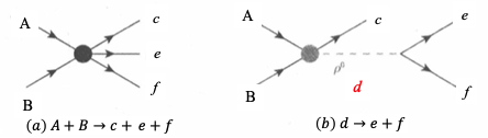
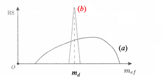
A final-state particle pair may be produced in two different ways. In the non-resonant case, the particles are produced directly, for example,
$$ A+B \to c+d+e. $$
Then the invariant mass of a selected pair, such as $c+d$, varies smoothly according to phase space. In the resonant case, an intermediate state is produced first and then decays:
$$ A+B \to c+R,\qquad R\to e+f. $$
Now the invariant mass of the pair $e+f$ clusters around the mass of the resonance $R$. This is the physical reason invariant-mass spectra are so useful: they distinguish smooth phase-space production from the production of an actual intermediate state.
Missing Mass
Missing mass is used when not all final-state particles are detected.
If the initial-state four-momentum is known and only part of the final state is measured, the missing four-momentum is defined as
$$ P_{\mathrm{miss}}=(P_A+P_B)-P_{\mathrm{detected}}. $$
The missing mass is then
$$ M_{\mathrm{miss}}^2=P_{\mathrm{miss}}^2. $$ So invariant mass and missing mass are closely related:
- invariant mass reconstructs a state from detected daughters;
- missing mass reconstructs an undetected particle or system from the known initial state and the measured remainder.
Both are direct applications of four-momentum conservation.
Example 1: Total Invariant Mass of the $3\alpha$ System
We consider the decay
$$ ^{12}\mathrm C^* \to \alpha+\alpha+\alpha. $$
For each event, the three alpha-particle four-vectors are reconstructed from the stored kinetic energies and angles. The total invariant mass is then
$$ M_{3\alpha}=\sqrt{(P_1+P_2+P_3)^2}. $$
The following code calculates the excitation energy of $^{12}\mathrm C^*$, $$ E_x(^{12}\mathrm C^*) = M_{3\alpha} - M(^{12}\mathrm C_{\mathrm{g.s.}}) $$
TCanvas *c = new TCanvas("c", "c", 700, 500);
%%cpp -d
const double m_alpha = 3.727379378;      // GeV

const double c12_threshold = 0.0072747;  // GeV = 7.2747 MeV
const double m_c12_gs = 3.0 * m_alpha - c12_threshold;

const double be8_gs_excess = 0.00009184; // GeV = 91.84 keV
const double m_be8_gs = 2.0 * m_alpha + be8_gs_excess;

TLorentzVector MakeAlphaP4(double T_mev, double theta_deg, double phi_deg)
{
    double T  = T_mev / 1000.0;   // MeV -> GeV
    double E  = T + m_alpha;
    double p  = std::sqrt(T * T + 2.0 * m_alpha * T);

    double th = theta_deg * TMath::DegToRad();
    double ph = phi_deg   * TMath::DegToRad();

    double px = p * std::sin(th) * std::cos(ph);
    double py = p * std::sin(th) * std::sin(ph);
    double pz = p * std::cos(th);

    return TLorentzVector(px, py, pz, E);
}
void excitation_energy_12c_from_3alpha()
{
    TFile *f = TFile::Open("direct_3alpha.root");
    TTree *tr = (TTree*)f->Get("events");

    double T_rest[3];
    double theta_rest[3];
    double phi_rest[3];
    double weight;

    tr->SetBranchAddress("T_rest", T_rest);
    tr->SetBranchAddress("theta_rest", theta_rest);
    tr->SetBranchAddress("phi_rest", phi_rest);
    tr->SetBranchAddress("weight", &weight);

    TH1F *h = new TH1F(
        "h",
        "Excitation energy of ^{12}C*;E_{x}(MeV);Counts",
        240, 0.0, 20.0
    );

    Long64_t nentries = tr->GetEntries();

    for (Long64_t i = 0; i < nentries; ++i) {
        tr->GetEntry(i);

        TLorentzVector p1 = MakeAlphaP4(T_rest[0], theta_rest[0], phi_rest[0]);
        TLorentzVector p2 = MakeAlphaP4(T_rest[1], theta_rest[1], phi_rest[1]);
        TLorentzVector p3 = MakeAlphaP4(T_rest[2], theta_rest[2], phi_rest[2]);

        double m3a = (p1 + p2 + p3).M();            // GeV
        double ex  = (m3a - m_c12_gs) * 1000.0;    // MeV

        h->Fill(ex, weight);
    }
    h->Draw("hist");
    c->Draw();
}
excitation_energy_12c_from_3alpha();
Example: Missing-Mass Reconstruction in the $3\alpha$ System
For a fully reconstructed $3\alpha$ event, one may define the missing mass against a selected alpha particle.
For example,
$$ M_{\mathrm{miss},1}^2=(P_{3\alpha}-P_1)^2. $$
Because
$$ P_{3\alpha}-P_1=P_2+P_3, $$
this missing mass is equal to the invariant mass of the complementary two-alpha subsystem:
$$ M_{\mathrm{miss},1}=m_{23}. $$
Similarly,
$$ M_{\mathrm{miss},2}=m_{13},\qquad M_{\mathrm{miss},3}=m_{12}. $$
To study the recoil two-alpha system relative to the $^{8}\mathrm{Be}$ ground state, we define the excitation energy
$$ E_x(^{8}\mathrm{Be}) = M_{\mathrm{miss}} - M(^{8}\mathrm{Be}_{\mathrm{g.s.}}). $$
For direct three-body decay, this missing-mass spectrum is expected to vary smoothly within the kinematically allowed region.
For sequential decay, the broad structure originates from the intermediate $^{8}\mathrm{Be}(2^+)$ resonance, while the smooth underlying background comes from the remaining nonresonant alpha-particle combinations.
void missing_mass_excitation_energy_be8()
{
    TFile *f1 = TFile::Open("direct_3alpha.root");
    TTree *tr1 = (TTree*)f1->Get("events");

    TFile *f2 = TFile::Open("sequential_3alpha.root");
    TTree *tr2 = (TTree*)f2->Get("events");

    double T_move[3];
    double theta_move[3];
    double phi_move[3];
    double weight;

    TH1F *h_dir = new TH1F(
        "h_dir",
        "Missing-mass excitation energy relative to ^{8}Be(g.s.);E_{x}(MeV);Counts",
        240, -0.5, 10.0
    );

    TH1F *h_seq = new TH1F(
        "h_seq",
        "Missing-mass excitation energy relative to ^{8}Be(g.s.);E_{x}(MeV);Counts",
        240, -0.5, 10.0
    );

    tr1->SetBranchAddress("T_move", T_move);
    tr1->SetBranchAddress("theta_move", theta_move);
    tr1->SetBranchAddress("phi_move", phi_move);
    tr1->SetBranchAddress("weight", &weight);

    Long64_t n1 = tr1->GetEntries();

    for (Long64_t i = 0; i < n1; ++i) {
        tr1->GetEntry(i);

        TLorentzVector p1 = MakeAlphaP4(T_move[0], theta_move[0], phi_move[0]);
        TLorentzVector p2 = MakeAlphaP4(T_move[1], theta_move[1], phi_move[1]);
        TLorentzVector p3 = MakeAlphaP4(T_move[2], theta_move[2], phi_move[2]);
        TLorentzVector p_total = p1 + p2 + p3;

        double ex1 = ((p_total - p1).M() - m_be8_gs) * 1000.0; // recoil against alpha 1
        double ex2 = ((p_total - p2).M() - m_be8_gs) * 1000.0; // recoil against alpha 2
        double ex3 = ((p_total - p3).M() - m_be8_gs) * 1000.0; // recoil against alpha 3

        h_dir->Fill(ex1, weight);
        h_dir->Fill(ex2, weight);
        h_dir->Fill(ex3, weight);
    }

    tr2->SetBranchAddress("T_move", T_move);
    tr2->SetBranchAddress("theta_move", theta_move);
    tr2->SetBranchAddress("phi_move", phi_move);
    tr2->SetBranchAddress("weight", &weight);

    Long64_t n2 = tr2->GetEntries();

    for (Long64_t i = 0; i < n2; ++i) {
        tr2->GetEntry(i);

        TLorentzVector p1 = MakeAlphaP4(T_move[0], theta_move[0], phi_move[0]);
        TLorentzVector p2 = MakeAlphaP4(T_move[1], theta_move[1], phi_move[1]);
        TLorentzVector p3 = MakeAlphaP4(T_move[2], theta_move[2], phi_move[2]);

        TLorentzVector p_total = p1 + p2 + p3;

        double ex1 = ((p_total - p1).M() - m_be8_gs) * 1000.0;
        double ex2 = ((p_total - p2).M() - m_be8_gs) * 1000.0;
        double ex3 = ((p_total - p3).M() - m_be8_gs) * 1000.0;

        h_seq->Fill(ex1, weight);
        h_seq->Fill(ex2, weight);
        h_seq->Fill(ex3, weight);
    }

    h_dir->SetLineColor(kBlue);
    h_seq->SetLineColor(kRed);

    c->Clear();
    gStyle->SetOptStat(0);

    h_seq->Draw("hist");
    h_dir->Draw("hist same");

    TLegend *leg = new TLegend(0.58, 0.72, 0.88, 0.88);
    leg->AddEntry(h_dir, "Direct", "l");
    leg->AddEntry(h_seq, "Sequential", "l");
    leg->Draw();
    c->Draw();
}
missing_mass_excitation_energy_be8()
Three-Body Decays and the Dalitz Plot
For a three-body decay,
$$ M\to 1+2+3, $$
the Dalitz plot is a two-dimensional way to represent the internal kinematics of the final state.
A standard construction is to choose two independent variables from the three pairwise invariant masses squared,
$$ m_{12}^2=(P_1+P_2)^2,\qquad m_{13}^2=(P_1+P_3)^2,\qquad m_{23}^2=(P_2+P_3)^2. $$
Since only two of them are independent, a Dalitz plot can be drawn, for example, as
$$ m_{12}^2 \ \text{vs.}\ m_{13}^2. $$
Each event is then represented by one point in the allowed kinematic region.
For a specific decay, one may also use an equivalent set of variables that is more convenient for the symmetry of the final state.
Example 4: Dalitz Plot of the $3\alpha$ Final State
For the $3\alpha$ final state, it is convenient to use Dalitz coordinates constructed from the kinetic energies of the three alpha particles in the move frame of the $3\alpha$ system.
Define the normalized kinetic-energy fractions
$$ \varepsilon_i=\frac{T_i}{T_1+T_2+T_3}, \qquad \varepsilon_1+\varepsilon_2+\varepsilon_3=1. $$
The Dalitz coordinates are taken as
$$ x=\sqrt{3}\,(\varepsilon_1-\varepsilon_2), \qquad y=2\varepsilon_3-\varepsilon_1-\varepsilon_2. $$
This is an alternative Dalitz-plot construction for the same three-body decay, chosen here because it makes the symmetry of the $3\alpha$ system more transparent.
For direct decay, the distribution is expected to populate the allowed region relatively smoothly.
For sequential decay, the Dalitz plot develops broad structures associated with the intermediate $^{8}\mathrm{Be}(2^+)$ state.
void dalitz_plot_3alpha()
{
    TFile *f1 = TFile::Open("direct_3alpha.root");
    TTree *tr1 = (TTree*)f1->Get("events");

    TFile *f2 = TFile::Open("sequential_3alpha.root");
    TTree *tr2 = (TTree*)f2->Get("events");

    double T_move[3];
    double theta_move[3];
    double phi_move[3];
    double weight;

    TH2F *h_dir = new TH2F(
        "h_dir",
        "Dalitz plot: direct decay;x;y",
        250, -1.4, 1.4,
        250, -1.4, 1.4
    );

    TH2F *h_seq = new TH2F(
        "h_seq",
        "Dalitz plot: sequential decay;x;y",
        250, -1.4, 1.4,
        250, -1.4, 1.4
    );

    tr1->SetBranchAddress("T_move", T_move);
    tr1->SetBranchAddress("theta_move", theta_move);
    tr1->SetBranchAddress("phi_move", phi_move);
    tr1->SetBranchAddress("weight", &weight);

    Long64_t n1 = tr1->GetEntries();

    for (Long64_t i = 0; i < n1; ++i) {
        tr1->GetEntry(i);

        double T1 = T_move[0];
        double T2 = T_move[1];
        double T3 = T_move[2];
        double Tsum = T1 + T2 + T3;

        if (Tsum <= 0.0) continue;

        double e1 = T1 / Tsum;
        double e2 = T2 / Tsum;
        double e3 = T3 / Tsum;

        double x = std::sqrt(3.0) * (e1 - e2);
        double y = 2.0 * e3 - e1 - e2;

        h_dir->Fill(x, y, weight);
    }

    tr2->SetBranchAddress("T_move", T_move);
    tr2->SetBranchAddress("theta_move", theta_move);
    tr2->SetBranchAddress("phi_move", phi_move);
    tr2->SetBranchAddress("weight", &weight);

    Long64_t n2 = tr2->GetEntries();

    for (Long64_t i = 0; i < n2; ++i) {
        tr2->GetEntry(i);

        double T1 = T_move[0];
        double T2 = T_move[1];
        double T3 = T_move[2];
        double Tsum = T1 + T2 + T3;

        if (Tsum <= 0.0) continue;

        double e1 = T1 / Tsum;
        double e2 = T2 / Tsum;
        double e3 = T3 / Tsum;

        double x = std::sqrt(3.0) * (e1 - e2);
        double y = 2.0 * e3 - e1 - e2;

        h_seq->Fill(x, y, weight);
    }
    gStyle->SetOptStat(0);

    delete c;
    TCanvas *c1 = new TCanvas("c1", "Dalitz direct", 700, 600);
    h_dir->Draw("colz");


    TCanvas *c2 = new TCanvas("c2", "Dalitz sequential", 700, 600);
    h_seq->Draw("colz");
}
dalitz_plot_3alpha();
c1->Draw();
c2->Draw();