$\gamma-\gamma$ 对称矩阵的整体减本底方法:Radware approach
本节讨论一种二维对称矩阵的整体减本底方法,它的基本思路是:
- 由二维 $\gamma-\gamma$ 矩阵得到 total projection;
- 将 total projection 近似分解为 peak component 和 background component;
- 根据这两个一维成分构造二维 background matrix;
- 从原始二维矩阵中扣除 background matrix;
- 在扣本底后的矩阵上进行开窗(gate),检查符合关系。
ROOT文件
本节继续使用 5.0 中得到的 addback 后数据文件:
eurica_addback.root
构建二维 $\gamma-\gamma$ 对称矩阵
二维 $\gamma-\gamma$ 矩阵的一个 bin $(E_i,E_j)$ 表示在同一个 prompt coincidence 中,两个 addback hit 的能量分别为 $E_i$ 和 $E_j$。
对于同一事件中的两个 addback hit,先计算时间差
$$ \Delta t = t_i - t_j. $$
若
$$ |\Delta t| < t_{\mathrm{prompt}}, $$
则认为这两个 hit 属于 prompt coincidence,并将其能量填入二维矩阵。
为了构造对称矩阵,每一个 $\gamma-\gamma$ pair 同时填入
$$ (E_i,E_j) $$
和
$$ (E_j,E_i). $$
这样得到的矩阵满足
$$ M_{ij}=M_{ji}. $$
下面的代码直接从 eurica_addback.root 构造二维对称矩阵。为了检查时间窗,同时保存一个对称填充的时间差谱 hdt_sym。这里 hdt_sym 只用于观察时间结构,不用于归一化。
%%cpp -d

#include <iostream>
#include <cmath>
#include <algorithm>

const int MAXHIT = 1024;

void make_symmetric_gg_matrix(const char *infile  = "eurica_addback.root",
                              const char *outfile = "eurica_ggmatrix.root",
                              int nbins = 1500,
                              double emax = 1530.0,
                              double emin = 30.0,
                              double dtPrompt = 180.0)
{
  TFile *fin = new TFile(infile);
  if (!fin || fin->IsZombie()) {
    std::cout << "cannot open " << infile << std::endl;
    return;
  }

  TTree *tree = (TTree*)fin->Get("tree");
  if (!tree) {
    std::cout << "cannot find tree" << std::endl;
    fin->Close();
    return;
  }

  int ahit;
  int aid[MAXHIT];
  double ae[MAXHIT];
  double at[MAXHIT];

  tree->SetBranchAddress("ahit", &ahit);
  tree->SetBranchAddress("aid", aid);
  tree->SetBranchAddress("ae", ae);
  tree->SetBranchAddress("at", at);

  TH1::SetDefaultSumw2(kTRUE);

  TH2D *hgg = new TH2D("hgg",
                       "#gamma-#gamma symmetric matrix;E_{x} (keV);E_{y} (keV)",
                       nbins, 0, emax,
                       nbins, 0, emax);

  TH1D *hdt_sym = new TH1D("hdt_sym",
                           "symmetric time difference spectrum;#Deltat (ns);counts",
                           800, -4000, 4000);

  Long64_t nentries = tree->GetEntries();

  for (Long64_t ientry = 0; ientry < nentries; ientry++) {

    tree->GetEntry(ientry);

    int nhit = std::min(ahit, MAXHIT);

    for (int i = 0; i < nhit; i++) {
      if (ae[i] < emin) continue;
      for (int j = i + 1; j < nhit; j++) {
        if (ae[j] < emin) continue;
        if (aid[i] == aid[j]) continue;

        double dt = at[i] - at[j];
        double adt = std::fabs(dt);

        hdt_sym->Fill(dt);
        hdt_sym->Fill(-dt);

        if (adt < dtPrompt) {

          hgg->Fill(ae[i], ae[j]);
          hgg->Fill(ae[j], ae[i]);

        }
      }
    }

    if (ientry % 100000 == 0) {
      std::cout << "processing " << ientry << " / " << nentries << "\r";
      std::cout.flush();
    }
  }

  std::cout << std::endl;

  TFile *fout = new TFile(outfile, "recreate");
  hdt_sym->Write();
  hgg->Write();
  fout->Close();

  fin->Close();

  std::cout << "symmetric gamma-gamma matrix saved to "
            << outfile << std::endl;
}
make_symmetric_gg_matrix();
processing 10300000 / 10370481
symmetric gamma-gamma matrix saved to eurica_ggmatrix.root
检查时间差分布和二维矩阵
TCanvas *c1 = new TCanvas("c1", "c1", 800, 700);

TFile *fg = new TFile("eurica_ggmatrix.root");

TH1D *hdt_sym = (TH1D*)fg->Get("hdt_sym");
TH2D *hgg = (TH2D*)fg->Get("hgg");
二维 $\gamma-\gamma$ 对称矩阵
%jsroot off
hgg->Draw("colz");
gPad->SetLogz();
c1->Draw();

Total projection 与一维本底分解
设二维对称矩阵为 $M_{ij}$。沿一个方向投影得到 total projection:
$$ P_i=\sum_j M_{ij}. $$
其中 $P_i$ 表示二维矩阵中与第 $i$ 个能量 bin 相关的总符合计数。
.L peaks.C
TCanvas *c2 = new TCanvas("c2", "c2", 1000, 600);
TH1D *hproj = hgg->ProjectionX("hproj");

hproj->SetTitle("total projection spectrum;E_{#gamma} (keV);counts");
peaks("hproj");
gPad->SetLogy();
c2->Draw();

Total projection 中既包含 full-energy peaks,也包含 Compton continuum 和 quasi-continuum。Radware approach 首先将 total projection 近似分解为
$$ P_i=p_i+b_i. $$
其中:
- $p_i$ 是第 $i$ 个 bin 中的 peak component;
- $b_i$ 是第 $i$ 个 bin 中的 background component。
这里的 $p_i$ 和 $b_i$ 不是对每一个物理峰逐峰拟合得到的结果,而是从 total projection 中估计出的平均 peak / background 成分。
使用 TSpectrum::Background() 估计一维本底。
其中:
hproj对应 $P_i$;hbg1d对应 $b_i$;hpeak1d对应 $p_i$。
TSpectrum::Background() 的参数需要通过图形检查。若本底线明显穿过强峰,说明本底估计过高;若本底线明显低于连续平台,说明本底估计过低。Radware approach 的效果首先取决于这一维分解是否合理。
TSpectrum *sp = new TSpectrum(500);

TH1D *hbg1d = (TH1D*)sp->Background(hproj, 6, "nosmoothing");
hbg1d->SetName("hbg1d");
hbg1d->SetTitle("1D background from total projection");

TH1D *hpeak1d = (TH1D*)hproj->Clone("hpeak1d");
hpeak1d->SetTitle("peak component of total projection");
hpeak1d->Add(hbg1d, -1.0);

TCanvas *c3 = new TCanvas("c3", "c3", 1100, 400);
c3->Divide(2,1);
c3->cd(1);
hproj->Draw();
hbg1d->SetLineColor(kRed);
hbg1d->Draw("same");
gPad->SetLogy();
c3->cd(2);
hpeak1d->SetLineColor(kBlack);
hpeak1d->Draw();
gPad->SetLogy();
c3->Draw();

Background matrix
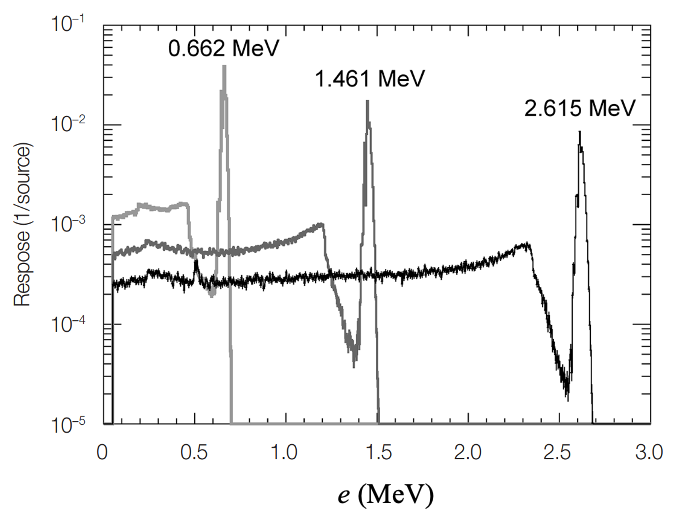
设真实 $\gamma$ 跃迁能量为 $E$,测量能量为 $e$。探测器响应函数记为
$$ R(e,E)=R_p(e,E)+R_b(e,E), $$
其中 $R_p$ 表示 full-energy peak response,$R_b$ 表示 background response。
若真实符合 $\gamma$ 对 $(E_1,E_2)$ 在当前实验条件下进入二维矩阵的权重为 $W(E_1,E_2)$,则实验二维符合谱为
$$ M(e_x,e_y) = \int dE_1dE_2\, W(E_1,E_2) R(e_x,E_1) R(e_y,E_2). $$
代入 $R=R_p+R_b$,二维谱可以分成
$$ M=M_{pp}+M_{pb}+M_{bp}+M_{bb}. $$
其中 $M_{pp}$ 表示两个方向都来自 full-energy peak 的真实符合,应该保留;而
$$ B_{\mathrm{exact}} = M_{pb}+M_{bp}+M_{bb} $$
是严格意义下的二维本底,因为它们至少有一个方向来自 background response。
Radware 本底矩阵
- D.C. Radford, Nucl. Instr. Meth. A361(1995)306
严格本底的计算需要知道真实符合关系 $W(E_1,E_2)$ 以及每条 $\gamma$ 的响应函数 $R_p$ 和 $R_b$,实际分析中通常无法做到。Radware 方法因此采用一个全局平均近似。
首先定义 total projection:
$$ P(e)=\int M(e,e')\,de', $$
并将其分成 peak 和 background 两部分:
$$ P(e)=p(e)+b(e). $$
这里 $P(e)$ 不是普通 singles spectrum,而是二维 $\gamma-\gamma$ 谱的边缘分布;$p(e)$ 和 $b(e)$ 分别表示这个边缘分布中的 peak 成分和 background 成分。
Radware 方法用 $p(e)$ 和 $b(e)$ 的一维平均形状近似二维本底中的三类贡献:
$$ M_{pb}(e_x,e_y) \approx \frac{p(e_x)b(e_y)}{T}, $$
$$ M_{bp}(e_x,e_y) \approx \frac{b(e_x)p(e_y)}{T}, $$
$$ M_{bb}(e_x,e_y) \approx \frac{b(e_x)b(e_y)}{T}, $$
其中
$$ T=\int P(e)\,de. $$
因此 Radware 本底矩阵为
$$ B_{\mathrm{RW}}(e_x,e_y) = \frac{ p(e_x)b(e_y) + b(e_x)p(e_y) + b(e_x)b(e_y) }{T}. $$
利用 $P(e)=p(e)+b(e)$,也可以写成
$$ B_{\mathrm{RW}}(e_x,e_y) = \frac{ P(e_x)P(e_y)-p(e_x)p(e_y) }{T}, $$
这个近似的物理含义是:Radware 方法不再逐条计算真实 $\gamma$ 的 Compton continuum 和 partner 关系,而是用 total projection 中的平均 peak/background 分布构造二维本底。因此,它是一种全局平均本底估计,而不是严格的二维响应函数计算。
- 上述方法可以推广到 3-fold,4-fold的矩阵
其他方法:
- G. Palameta and J.C. Waddington, Nucl. Instr. Meth. A234(1985)476
- TSpectrum2的Background()方法
%%cpp -d

#include <iostream>
#include <cmath>
#include <algorithm>

void make_radware_matrix(const char *infile  = "eurica_ggmatrix.root",
                         const char *matrixName = "hgg",
                         const char *outfile = "eurica_gg_radware.root",
                         int bgIter = 6)
{
  TFile *fin = new TFile(infile);
  if (!fin || fin->IsZombie()) {
    std::cout << "cannot open " << infile << std::endl;
    return;
  }

  TH2D *hgg = (TH2D*)fin->Get(matrixName);
  if (!hgg) {
    std::cout << "cannot find matrix " << matrixName << std::endl;
    fin->Close();
    return;
  }

  TH1::SetDefaultSumw2(kTRUE);

  TH1D *hproj = hgg->ProjectionX("hproj");
  hproj->SetTitle("total projection spectrum;E_{#gamma} (keV);counts");

  TSpectrum *sp = new TSpectrum(500);

  TH1D *hbg1d = (TH1D*)sp->Background(hproj, bgIter, "nosmoothing");
  hbg1d->SetName("hbg1d");
  hbg1d->SetTitle("1D background from total projection");

  TH1D *hpeak1d = (TH1D*)hproj->Clone("hpeak1d");
  hpeak1d->SetTitle("1D peak component from total projection");
  hpeak1d->Add(hbg1d, -1.0);

  int nx = hgg->GetNbinsX();
  int ny = hgg->GetNbinsY();

  TH2D *hggb = (TH2D*)hgg->Clone("hggb_radware");
  hggb->Reset();
  hggb->SetTitle("Radware background matrix;E_{x} (keV);E_{y} (keV)");

  TH2D *hggmat = (TH2D*)hgg->Clone("hgg_radware");
  hggmat->SetTitle("background-subtracted #gamma-#gamma matrix;E_{x} (keV);E_{y} (keV)");

  double T = hproj->Integral();

  for (int ix = 1; ix <= nx; ix++) {

    double Pi = hproj->GetBinContent(ix);
    double pi = hpeak1d->GetBinContent(ix);

    if (Pi < 0) Pi = 0;
    if (pi < 0) pi = 0;
    if (pi > Pi) pi = Pi;

    for (int iy = 1; iy <= ny; iy++) {

      double Pj = hproj->GetBinContent(iy);
      double pj = hpeak1d->GetBinContent(iy);

      if (Pj < 0) Pj = 0;
      if (pj < 0) pj = 0;
      if (pj > Pj) pj = Pj;

      double Bij = 0.0;

      if (T > 0) {
        Bij = (Pi * Pj - pi * pj) / T;
      }

      if (Bij < 0) Bij = 0;

      hggb->SetBinContent(ix, iy, Bij);
      hggb->SetBinError(ix, iy, std::sqrt(Bij));
    }
  }

  hggmat->Add(hggb, -1.0);

  TFile *fout = new TFile(outfile, "recreate");

  hgg->Write("hgg_input");
  hproj->Write();
  hbg1d->Write();
  hpeak1d->Write();
  hggb->Write();
  hggmat->Write();

  fout->Close();
  fin->Close();

  std::cout << "Radware background-subtracted matrix saved to "
            << outfile << std::endl;
}
make_radware_matrix();
Radware background-subtracted matrix saved to eurica_gg_radware.root
检查 background matrix 和扣本底矩阵
TFile *fr = new TFile("eurica_gg_radware.root");

TH2D *hgg_input = (TH2D*)fr->Get("hgg_input");
TH2D *hggb_radware = (TH2D*)fr->Get("hggb_radware");
TH2D *hgg_radware = (TH2D*)fr->Get("hgg_radware");
c1->Clear();
hggb_radware->Draw("colz");
gPad->SetLogy(0);
gPad->SetLogz();
c1->Draw();

Background matrix 应主要反映连续本底区域的整体强度分布,而不应产生尖锐孤立的 peak-peak 结构。
再看扣本底后的二维矩阵:
hgg_radware->Draw("colz");
gPad->SetLogz();
c1->Draw();

减本底后应观察到:
- 连续平台降低;
- 强的真实符合点保留;
- 由 Compton continuum 产生的横向或纵向本底减弱;
- 统计较弱的位置可能出现接近零或负计数的波动。
扣本底后的矩阵不能简单理解为“只剩真实符合”。它只是降低了连续本底的平均贡献。
比较扣本底前后的投影谱:
TCanvas *c2 = new TCanvas("c2","c2",1000,600);
Warning in <TCanvas::Constructor>: Deleting canvas with same name: c2
TH1D *hproj_raw = hgg_input->ProjectionX("hproj_raw");
TH1D *hproj_net = hgg_radware->ProjectionX("hproj_net");

hproj_raw->SetLineColor(kBlack);
hproj_net->SetLineColor(kRed);

hproj_raw->Draw("hist");
hproj_net->Draw("hist same");

gPad->SetLogy();
c2->Draw();

扣本底后,连续平台应降低,主要的全能峰应保留。若主要峰明显被削弱,说明一维本底估计可能过高;若连续平台几乎没有变化,说明本底估计可能过低。
对于扣本底后的 bin,
$$ N_{\mathrm{net}} = N_{\mathrm{raw}}-N_{\mathrm{bkg}}. $$
其统计不确定度近似为
$$ \sigma_{N_{\mathrm{net}}} \simeq \sqrt{ \sigma_{N_{\mathrm{raw}}}^2 + \sigma_{N_{\mathrm{bkg}}}^2 }. $$
因此,弱峰在扣本底后的相对不确定度可能变大,不能只凭二维图上的颜色判断其为真实符合。
只有尽量减少本底贡献,才能确认弱关联的gamma之间的符合关系
途径:每个探测器加入anti-compton shield;通过加入其它探测器的符合,压制本底...
void zoom2D(TH2D *h,
            double xmin, double xmax,
            double ymin, double ymax,
            const char *opt = "colz")
{
  h->GetXaxis()->SetRangeUser(xmin, xmax);
  h->GetYaxis()->SetRangeUser(ymin, ymax);
  h->Draw(opt);
  //gPad->SetLogz();
  gPad->Update();
}
TCanvas *c5 = new TCanvas("c5","c5",900,300);
c5->Divide(3,1);
c5->cd(1);
zoom2D(hgg_input, 50, 200, 50, 200);

c5->cd(2);
zoom2D(hggb_radware, 50, 200, 50, 200);

c5->cd(3);
zoom2D(hgg_radware, 50, 200, 50, 200);
c5->Draw();

减本底的矩阵中,来源于133Ba的(80,80)的符合清晰可见,而其他有偶然本底导致的交叉点(80,121),(121,80)消失。
在扣本底矩阵上进行开窗(gate)
定义一个通用 gate 函数。在二维对称矩阵中,如果在 $x$ 轴某个能量范围开 gate,则投影到 $y$ 轴。
TH1D* gate_gg(TH2D *hgg,
              double gateE,
              double gateWidth = 2.0,
              double xmax = 1300.0)
{
  static int igate = 0;
  igate++;

  hgg->GetXaxis()->SetRangeUser(0, xmax);
  hgg->GetYaxis()->SetRangeUser(0, xmax);

  int bin1 = hgg->GetXaxis()->FindBin(gateE - gateWidth);
  int bin2 = hgg->GetXaxis()->FindBin(gateE + gateWidth);

  TString hname;
  hname.Form("gate_%.1f_keV_%04d", gateE, igate);

  TH1D *hg = hgg->ProjectionY(hname, bin1, bin2);

  hg->SetTitle(Form("gated on %.1f keV;E_{#gamma} (keV);counts",gateE));

  hg->GetXaxis()->SetRangeUser(0, xmax);

  peaks(hname);

  return hg;
}
以 $121.8\,\mathrm{keV}$ 为例。先在原始矩阵中开 gate:
c2->Clear();
TH1D *h121_raw = gate_gg(hgg_input, 121.8, 2.0);
gPad->SetLogy(0);
c2->Draw();

再在 Radware 扣本底后的矩阵中开 gate:
c2->Clear();
TH1D *h121_net = gate_gg(hgg_radware, 121.8, 2.0);
gPad->SetLogy(0);
c2->Draw();

比较两张 gate 谱时,应看到原始 gate 谱中的连续平台在扣本底后降低,而与 $121.8\,\mathrm{keV}$ 有真实级联关系的峰仍然保留。弱峰是否可信,需要结合统计误差和反向 gate 检查。
用 $^{133}\mathrm{Ba}$ 检查符合关系
本实验源包含 $^{152}\mathrm{Eu}$ 和 $^{133}\mathrm{Ba}$。在扣本底后的二维矩阵上,可以利用 $^{133}\mathrm{Ba}$ 的已知级联关系检查矩阵是否合理。

常见的 $^{133}\mathrm{Ba}$ $\gamma$ 能量包括
$$ 53,\ 80,\ 160,\ 223,\ 276,\ 302,\ 356,\ 383\ \mathrm{keV}. $$
根据衰变纲图,可以预期不同 gate 中是否出现对应峰。下面用 O 表示预期有符合,用 x 表示预期没有明显符合。
| gate \ peak | $80$ | $160$ | $223$ | $302$ | $383$ | $53$ | $276$ | $356$ |
|---|---|---|---|---|---|---|---|---|
| $80$ | O | x | O | O | x | O | O | O |
| $223$ | O | O | x | x | x | O | x | x |
| $160$ | x | x | O | x | x | O | O | x |
| $302$ | O | x | x | x | x | O | x | x |
| $383$ | x | x | x | x | x | O | x | x |
| $53$ | O | O | O | O | O | x | x | x |
| $276$ | O | O | x | x | x | x | x | x |
| $356$ | O | x | x | x | x | x | x | x |
逐个开 gate:
TH1D *g80 = gate_gg(hgg_radware, 80.0, 2.0, 400);
c2->Draw();

TH1D *g223 = gate_gg(hgg_radware, 223.0, 2.0, 400);
c2->Draw();

TH1D *g160 = gate_gg(hgg_radware, 160.0, 2.0, 400);
c2->Draw();

g160:80附近有很明显峰结构,而在g80:160附近没有峰结构。可以基本断定80和160没有符合关系。参照[68]的右侧二维图的(80,160)附近结构。
c2->Clear();
TH1D *g302 = gate_gg(hgg_radware, 302.0, 2.0, 400);
c2->Draw();

c2->Clear();
TH1D *g383 = gate_gg(hgg_radware, 383.0, 2.0, 400);
c2->Draw();

c2->Clear();
TH1D *g53 = gate_gg(hgg_radware, 53.0, 2.0, 400);
c2->Draw();

c2->Clear();
TH1D *g276 = gate_gg(hgg_radware, 276.0, 2.0, 400);
c2->Draw();

c2->Clear();
TH1D *g356 = gate_gg(hgg_radware, 356.0, 2.0, 400);
c2->Draw();

检查符合关系时不要只看一个方向。一个候选符合关系至少应通过反向 gate 检查。例如,若 gate(160) 中出现 $80\,\mathrm{keV}$ 峰,还应检查 gate(80) 中是否存在 $160\,\mathrm{keV}$ 峰。
同时还要考虑低能探测效率、中间分支、峰面积显著性、summing peak 和 X-ray 干扰。二维矩阵最直接回答的问题是:两条 $\gamma$ 射线是否属于同一次级联退激过程。完整能级纲图还需要结合能量和关系、相对强度、效率修正、内转换、角关联和偏振等信息。
Radware 方法的局限性
Radware 方法的优点是可以从二维 $\gamma-\gamma$ 矩阵本身出发,利用 total projection 构造一个全局本底矩阵。这样可以避免对每一条 $\gamma$ 峰逐一开窗扣本底,在峰密度较高、级联关系较复杂的核谱学分析中很实用。
但是,Radware 方法不是严格的二维探测器响应计算,而是一种全局平均近似。它的局限性主要来自两个方面。
1. 全局平均假设不一定适合局部本底
Radware 方法隐含的基本假设是:某个局部本底区域所对应的符合 $\gamma$ 射线分布,可以用整个二维矩阵的 total projection 来近似。
这个假设在平均意义上有一定合理性。因为 total projection 确实反映了当前矩阵中所有 $\gamma-\gamma$ 符合关系的总体分布。但是,对于某一个具体的本底区域,这个近似不一定准确。
例如,某一段连续本底可能主要来自少数几条强 $\gamma$ 射线的 Compton 散射。这些强 $\gamma$ 射线在真实能级级联中只和特定的几条 $\gamma$ 射线符合。此时,这个局部本底对应的符合投影谱不一定和整个 total projection 的形状相同。
如果 Radware 方法仍然使用全局 total projection 来估计这个局部本底,就可能把一些实际上无关的强峰也作为本底结构扣掉。这样在扣本底后的二维谱中,就可能出现负本底、负峰或负的水平线、垂直线。
因此,Radware 扣本底后的负结构通常不应理解为物理上的负强度,而应理解为全局平均本底估计在局部区域发生了过扣。
2. 多反应道混合会加重过扣
在实际 in-beam $\gamma$ 谱学实验中,二维矩阵常常不是来自单一反应道,而是多个反应道、多个残余核、多个级联体系的叠加。
这时,total projection 也变成了多个反应道的混合谱。它包含了不同核素、不同级联分支和不同反应道的强峰。
问题在于:某一个局部本底区域可能主要来自其中一个反应道,但 Radware 方法却使用所有反应道混合后的 total projection 来估计本底。这样,其他反应道中的强峰也会被带入本底矩阵。
这些强峰本来可能和当前局部本底没有真实符合关系,但在扣本底时却被当作本底的一部分扣除。结果就容易在扣本底后的二维谱中形成负峰或负线。
因此,多反应道混合会削弱 total projection 的物理代表性,使 Radware 的全局平均近似更容易失效。这个问题在 fusion-evaporation 反应、高峰密度谱、反应道选择不干净的数据中尤其明显。
3. 如何部分改善
Radware 方法本身不能区分不同反应道。为了减小过扣,应尽量在构造二维矩阵或本底矩阵之前减少反应道混合。
可以根据实验条件进行筛选,例如:
- 粒子 gate;
- recoil gate 或 mass gate;
- prompt/delayed time gate;
- multiplicity 条件;
- 已知强 $\gamma$ transition gate;
- 与目标核素相关的符合条件。
筛选后的矩阵更接近单一反应道或单一物理过程。此时 total projection 更有可能代表该矩阵中局部本底的平均符合 $\gamma$ 分布,Radware 扣本底也会更稳定。
对于关键的 $\gamma$ 峰和关键符合关系,还应结合峰旁窗方法进行检查。峰旁窗方法直接利用峰附近的本底区域估计峰下本底,局部性更强。在孤立峰或本底较平滑的情况下,它通常比全局 Radware 方法更直观,也更适合验证某一条具体符合关系。
因此,Radware 方法适合用于全局二维矩阵的初步本底处理;而对于重要的弱峰、新能级或可疑符合关系,应结合反应道筛选、峰旁窗方法、double gate 等更有物理选择性的手段进行复核。
关于偶然符合
Radware approach 主要处理 Compton continuum 和 quasi-continuum 形成的连续本底,不等同于时间偶然符合扣除。
在本节代码中,二维矩阵由 prompt 时间窗内的 $\gamma-\gamma$ pair 构成。如果实验计数率较低,偶然符合通常只是较小修正,可以先观察 Radware 减本底后的效果。
在高计数率束流实验中,低能区可能出现强 X-ray。例如 Au、Pb 等材料被束流激发后,会产生特征 X-ray。这些 X-ray 与反应产物的 $\gamma$ 射线通常没有真实级联关系,但可能由于计数率高而进入 prompt 窗,形成偶然符合。
此时,应进一步构造 accidental matrix。设:
PAM:prompt window 内的矩阵,包含 prompt 和 accidental;AM:prompt window 外的 accidental matrix;PM:扣除偶然符合后的 prompt matrix。
若 prompt 时间窗宽度为 $\Delta t_P$,accidental 时间窗总宽度为 $\Delta t_A$,则
$$ PM = PAM - \frac{\Delta t_P}{\Delta t_A}AM. $$
在实际分析中,通常先进行 accidental subtraction,再对扣除偶然符合后的 prompt matrix 做 Radware background subtraction。
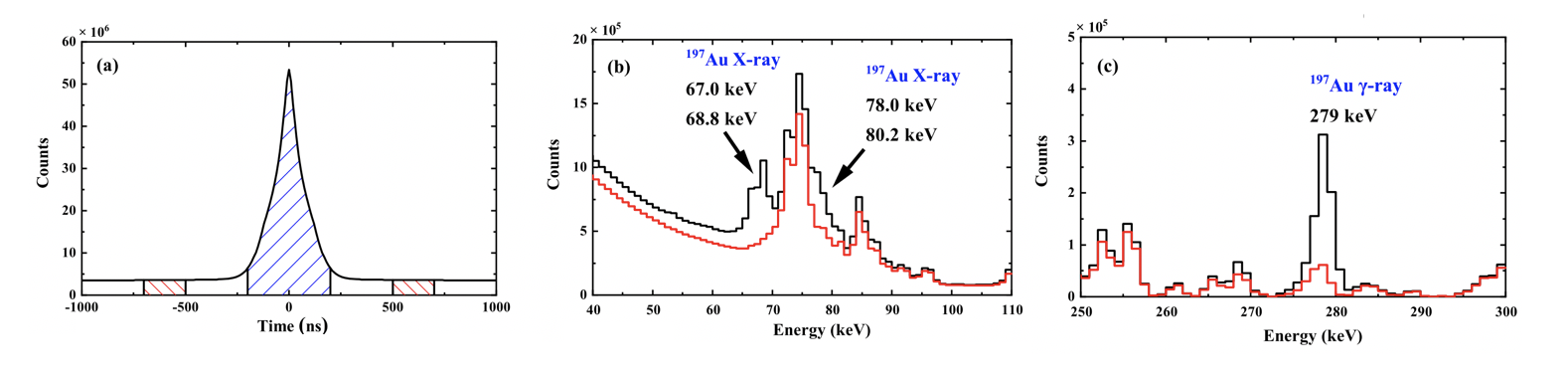
原则上,偶然符合时间窗的选择应紧挨着符合时间窗的两个对称时间窗。图b和c展示了扣除偶然符合前后的投影谱对比图。黑色表示未扣除偶然符合的投影谱,而红色表示扣除偶然符合后的投影谱。可以看出,通过偶然符合的扣除,197Au的X射线影响大大减少。
作业:
- 参考 5.1 中的 $^{152}$Eu 简化纲图,对同一分支内较强的 $\gamma$ 跃迁开窗,验证它们之间的符合关系。所有符合关系应用反向开窗交叉检查。
- 验证左右两分支的gamma之间没有符合关系,并在的简化纲图基础上进行扩展。