$\gamma - \gamma$ coincidence
在核结构实验中,激发态原子核通常通过发射 $\gamma$ 射线退激。如果退激过程经过若干中间能级,就会产生一组具有时间关联的级联 $\gamma$ 射线。实验上如果只看一维 $\gamma$ 能谱,不同核素、不同能级跃迁、随机本底、康普顿散射和偶然符合都会混在一起,很多弱跃迁并不容易识别。
$\gamma$-$\gamma$ 符合分析利用的是同一次核退激过程中不同 $\gamma$ 射线之间的时间关联。若两条 $\gamma$ 射线属于同一级联过程,它们应当在探测器时间分辨范围内表现为 prompt coincidence。通过这种时间关联,可以选择与某一条 $\gamma$ 射线符合的其他跃迁,从而突出真实级联关系,压低随机本底,并为建立能级纲图提供依据。
Data
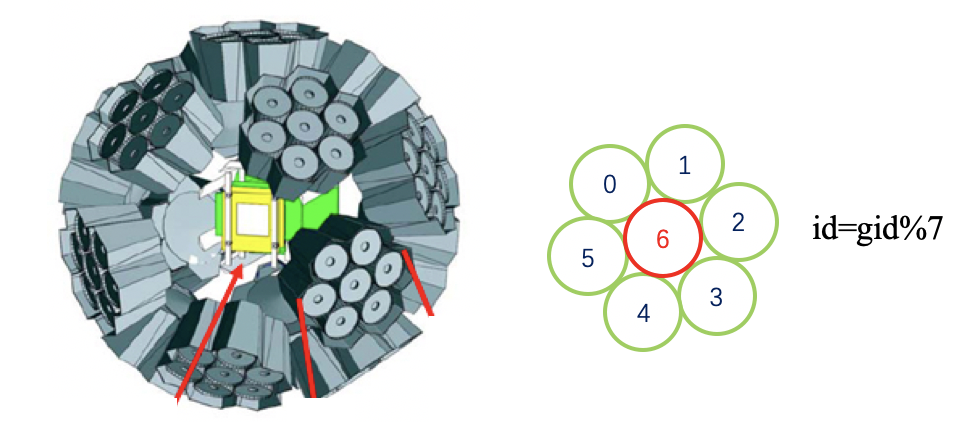
- EURICA comprises 12 Euroball IV HPGe cluster detectors, each with seven tapered hexagonal high-purity germanium (HPGe) crystals (84 crystals total across 12 cryostats)
Source: $^{152}Eu+^{133}Ba$
Detectors: Eurica Array: 12 Cluster Detectors
Electronics: 100Mhz, 14bit DGF-4C digitizer: energy , time 25ns/bin
Trigger: 1kHz Clock
Energy & time window: $100\mu s$ before trigger.
timing: leading edge discrimination for fast trigger.
- Data
- eurica.root TTree branch 为:
ghit
gid[ghit]
ge[ghit]
gt[ghit]
其中:
ghit:当前 entry 中原始晶体 hit 数;gid:晶体编号;ge:晶体能量;gt:晶体时间。
所有探测器之间的time delay已经对齐。
文件中也存在原始 addback branch:
ahit
aid[ahit]
ae[ahit]
at[ahit]
但是在本讲义后续处理中,不使用原文件中的 addback branch。后续 addback 分支由根据相邻探测单元关系生成(作业)。
TCanvas *c1 = new TCanvas("c1","c1");
TFile *fin = new TFile("eurica.root");
TTree *tree = (TTree*) fin->Get("tree");
Detector Id vs. Crystal ID
- Cluster ID:
int(gid/7) - Segment ID:
gid%7
tree->Draw("int(gid%7):int(gid/7)>>(12,0,12,7,0,7)","","colz");
c1->SetLogz(0);
c1->Draw();
tree->Scan("ge:gt:int(gid/7):gid%7","ghit==5","",50,1);
***********************************************************************
*    Row   * Instance *        ge *        gt * int(gid/7 *     gid%7 *
***********************************************************************
*       12 *        0 * 226.25437 * -46627.89 *         4 *         1 *
*       12 *        1 * 567.01922 * -70217.25 *         4 *         5 *
*       12 *        2 * 302.89921 * -52674.52 *         6 *         1 *
*       12 *        3 * 346.14300 * -39411.89 *        10 *         4 *
*       12 *        4 * 45.550980 * -54797.09 *        11 *         1 *
*       19 *        0 * 59.254901 * -44431.59 *         5 *         2 *
*       19 *        1 * 1271.8818 * -29141.77 *         6 *         0 *
*       19 *        2 * 75.999449 * -29302.45 *         9 *         0 *
*       19 *        3 * 121.50764 * -2130.173 *         9 *         4 *
*       19 *        4 * 84.346446 * -46206.87 *        11 *         2 *
*       47 *        0 * 91.955435 * -52516.33 *         4 *         3 *
*       47 *        1 * 149.63850 * -52494.53 *         4 *         4 *
*       47 *        2 * 114.82721 * -52616.77 *         4 *         6 *
*       47 *        3 * 235.44577 * -5468.176 *         6 *         3 *
*       47 *        4 * 46.279217 * -14524.26 *        11 *         1 *
***********************************************************************
==> 15 selected entries
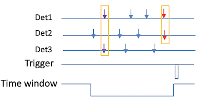
Event building
从 tree->Scan 的输出可以看到,一条 entry 中可能包含多个 hit。这些 hit 按 gid 升序排列,而不是按时间顺序排列。因此,原始 ROOT tree 中的一条 entry 不能直接看成一个物理 event。
本实验采用 1 kHz clock trigger。每次 trigger 记录触发前 $100~\mu\mathrm{s}$ 时间范围内的探测器命中信息。因此,一条 entry 实际上对应一个 $100~\mu\mathrm{s}$ 的 readout frame。在这样一个 frame 中,可能同时包含多个不同的时间结构:有的 event 中只有一个晶体记录到一个 $\gamma$ hit,有的 event 中多个晶体记录到来自同一次退激过程的级联 $\gamma$ hit。
γ₁
γ₁, γ₂
γ₁
γ₁, γ₂, γ₃
其中,single-$\gamma$ event 表示一个物理过程中只记录到一个 $\gamma$ hit;multi-$\gamma$ 事件 表示一个物理过程中记录到多个 $\gamma$ hit。为了进行后续 $\gamma$-$\gamma$ 符合分析,需要先根据 hit 的时间关系,把一个 readout frame 重新拆分为若干个 事件。这一步称为事件组装(event building)。
本节采用 fixed-window 方法进行 event building。首先将一个 entry 内所有 hit 按 gt 从小到大排序,然后从时间最早的未使用 hit 开始,打开一个固定宽度的 event window。若该 hit 的时间为 $t_{\mathrm{start}}$,则所有满足
$$ t_{\mathrm{start}} \leq t_i < t_{\mathrm{start}} + \Delta t_{\mathrm{event}} $$
的 hit 都放入同一个事件。第一个落在窗口外的 hit 作为下一个事件的起点。重复这一过程,直到当前 entry 中所有 hit 都被处理完。
start: t₀
window: t₀ to t₀ + Δtevent
γ₁
start: t₁
window: t₁ to t₁ + Δtevent
γ₁, γ₂
start: t₃
window: t₃ to t₃ + Δtevent
γ₁, γ₂, γ₃
event building window 的选择需要兼顾两个因素。窗口不能太窄,否则可能在事件组装阶段就把来自同一物理过程的 $\gamma$ hit 分到不同事件中;窗口也不能太宽,否则一个 $100~\mu\mathrm{s}$ frame 中相隔较远、彼此独立的 hit 会被错误地合并到同一个事件中。
在本实验数据中,放射源强度不高,随机堆积并不严重。后续 prompt $\gamma$-$\gamma$ 符合的时间尺度约为几百 ns。因此,这里选取一个相对宽松、但仍远小于 $100~\mu\mathrm{s}$ readout frame 的窗口:
$$ \Delta t_{\mathrm{event}} = 3~\mu\mathrm{s}. $$
即
$$ t_{\mathrm{start}} \leq t_i < t_{\mathrm{start}} + 3~\mu\mathrm{s}. $$
后续研究 prompt $\gamma$-$\gamma$ 符合时,还需要根据 time walk correction 后的时间差分布选择更窄的 prompt coincidence window。由于 $3~\mu\mathrm{s}$ 的 event building window 明显宽于后续 prompt coincidence window,一般不会因为后续的 time correction 而重新改变 event 的基本分组。
需要注意的是,fixed-window 方法仍然存在边界效应。如果某些原本属于同一物理过程的 hit 恰好位于窗口边界附近,它们仍可能在 event building 阶段被分到不同事件中。采用 $3~\mu\mathrm{s}$ 可以降低这种影响,但不能完全消除。
实际分析中也可以采用其他事件组装方法。
Gap-based event building 按照相邻 hit 的时间间隔判断是否属于同一个事件:
$$ t_i - t_{i-1} < \Delta t_{\mathrm{event}}. $$
如果相邻 hit 的时间间隔小于给定阈值,就继续放入当前事件;如果时间间隔超过阈值,则开始新的事件。
γ₁ → γ₂
small gap
γ₁ → γ₂ → γ₃
small gaps
这种方法不容易切开时间上相邻的 hit,但高计数率下可能出现 chain effect,即一串彼此间隔不大的 hit 被连成一个过长事件。
Fixed window with overlap 仍然使用 fixed window,但在相邻窗口之间保留一定重叠区。边界附近的 hit 可以先被两个窗口共同检查,后续再根据具体规则决定最终归属。
γ₁, γ₂
γ₃
γ₃, γ₄
这种方法可以减小边界附近相关 hit 被切开的概率,但后续需要处理重复归属和重复计数问题。
如果实验中有明确的物理 trigger 或参考探测器,还可以采用 reference-trigger event building。此时以参考时间 $T_0$ 为中心建立事件:
$$ T_0-\Delta t_1 < t_i < T_0+\Delta t_2. $$
γ
T₀ - Δt₁ ← T₀ → T₀ + Δt₂
γ₁, γ₂, γ₃
γ
本节数据来自 clock trigger 源实验,没有逐事件物理 trigger,因此采用 fixed-window event building。
生成 event-built ROOT 文件
下面的宏将原始 eurica.root 中的 $100~\mu\mathrm{s}$ frame 重新组装为事件,并保存为新的 ROOT 文件:
eurica_event.root
%%cpp -d

// build_event_tree.C

#include <iostream>
#include <map>

const int MAXHIT = 1024;

struct GammaHit {
  int gid;
  double ge;
};

void build_event_tree()
{
  const double eventWindow = 3000.0; // 3 μs, unit: ns

  TFile *fin = new TFile("eurica.root");
  TTree *tin = (TTree*)fin->Get("tree");

  int ghit;
  int gid_in[MAXHIT];
  double ge_in[MAXHIT];
  double gt_in[MAXHIT];

  tin->SetBranchAddress("ghit", &ghit);
  tin->SetBranchAddress("gid", gid_in);
  tin->SetBranchAddress("ge", ge_in);
  tin->SetBranchAddress("gt", gt_in);

  TFile *fout = new TFile("eurica_event.root", "recreate");
  TTree *tout = new TTree("tree", "event-built tree");

  int o_ghit;
  int o_gid[MAXHIT];
  double o_ge[MAXHIT];
  double o_gt[MAXHIT];

  tout->Branch("ghit", &o_ghit, "ghit/I");
  tout->Branch("gid", o_gid, "gid[ghit]/I");
  tout->Branch("ge", o_ge, "ge[ghit]/D");
  tout->Branch("gt", o_gt, "gt[ghit]/D");

  Long64_t nentries = tin->GetEntries();

  for (Long64_t ientry = 0; ientry < nentries; ++ientry) {

    tin->GetEntry(ientry);

    // key: gt
    // value: GammaHit(gid, ge)
    // multimap is used because different hits may have the same gt.
    std::multimap<double, GammaHit> timeHit;

    for (int i = 0; i < ghit; ++i) {

      GammaHit hit;
      hit.gid = gid_in[i];
      hit.ge = ge_in[i];

      timeHit.insert(std::make_pair(gt_in[i], hit));
    }

    std::multimap<double, GammaHit>::iterator it = timeHit.begin();

    while (it != timeHit.end()) {

      double tstart = it->first;
      double tend = tstart + eventWindow;

      o_ghit = 0;

      while (it != timeHit.end()) {

        double t = it->first;

        if (t >= tend) {
          break;
        }

        GammaHit hit = it->second;

        o_gid[o_ghit] = hit.gid;
        o_ge[o_ghit] = hit.ge;
        o_gt[o_ghit] = t;

        ++o_ghit;
        ++it;
      }

      tout->Fill();
    }
  }

  fout->cd();
  tout->Write();
  fout->Close();
  fin->Close();

  std::cout << "event-built file saved to eurica_event.root" << std::endl;
}
build_event_tree();
event-built file saved to eurica_event.root
打开新文件:
TFile *fin = new TFile("eurica_event.root");
TTree *tree = (TTree*) fin->Get("tree");
检查新的 event 结构:
tree->Scan("ghit:gid:ge:gt","","",10,0);
***********************************************************************
*    Row   * Instance *      ghit *       gid *        ge *        gt *
***********************************************************************
*        0 *        0 *         1 *         2 * 93.738894 * -67464.41 *
*        1 *        0 *         1 *        14 * 513.18847 * -38597.27 *
*        2 *        0 *         1 *        76 * 900.86628 * -16106.90 *
*        3 *        0 *         2 *        48 * 191.77148 * -11559.15 *
*        3 *        1 *         2 *        41 * 255.53136 * -11530.38 *
*        4 *        0 *         1 *        78 * 252.57337 * -52075.91 *
*        5 *        0 *         1 *        38 * 355.39204 * -17058.86 *
*        6 *        0 *         2 *        80 * 595.97674 * -84263.73 *
*        6 *        1 *         2 *        79 * 679.46405 * -84233.31 *
*        7 *        0 *         3 *        24 * 69.567794 * -23329.60 *
*        7 *        1 *         3 *        22 * 721.78308 * -23301.26 *
*        7 *        2 *         3 *        27 * 187.30067 * -23277.87 *
*        8 *        0 *         2 *        28 * 166.66361 * -17738.86 *
*        8 *        1 *         2 *        37 * 856.34057 * -17667.32 *
*        9 *        0 *         2 *        44 * 257.20985 * -5065.583 *
*        9 *        1 *         2 *        41 *  121.9316 * -5041.272 *
***********************************************************************
event multiplicity:
- 如果大多数事件的
ghit不高,说明在当前源强下 $3~\mu\mathrm{s}$ fixed window 没有造成明显 pile-up。如果ghit分布出现很长的高 multiplicity 尾部,则需要重新检查 event building window 是否过宽。
tree->Draw("ghit>>hghit(10,0,20)");
c1->SetLogy();
c1->Draw();
Check high-multiplicity events
完成 event building 后,需要检查 ghit 较大的事件。正常的放射源 $\gamma$-$\gamma$ 符合事件通常 multiplicity 不会很高。如果发现 ghit>5 的事件在时间上高度集中,而对应的 gid 又分布在许多不同探测器单元中,这类事件很可能不是来自真实的核退激过程,而是探测器系统中的公共干扰噪声或电子学噪声。
这类高 multiplicity 事件会在后续 $\gamma$-$\gamma$ 矩阵中引入大量虚假组合,因此应在分析中去除。一个简单处理方法是在 event building 阶段只保存 ghit<=5 的事件。
在代码中将 tout->Fill();改为:
if (o_ghit < 5) {
  tout->Fill();
}
tree->Scan("ghit:int(gid/7):gid%7:ge:gt","ghit>10","",200000,0);
***********************************************************************************
*    Row   * Instance *      ghit * int(gid/7 *     gid%7 *        ge *        gt *
***********************************************************************************
*   126521 *        0 *        15 *        11 *         1 * 160.50687 * -40134.72 *
*   126521 *        1 *        15 *         4 *         3 * 274.79625 * -40141.03 *
*   126521 *        2 *        15 *         8 *         0 * 155.69960 * -40077.67 *
*   126521 *        3 *        15 *         1 *         0 * 1354.3438 * -40137.15 *
*   126521 *        4 *        15 *         9 *         3 *    178.24 * -40062.61 *
*   126521 *        5 *        15 *        11 *         2 * 498.58192 * -40102.45 *
*   126521 *        6 *        15 *         0 *         4 * 216.90833 * -40036.18 *
*   126521 *        7 *        15 *         9 *         6 * 323.25703 * -40059.58 *
*   126521 *        8 *        15 *         1 *         2 * 1504.8202 * -40090.74 *
*   126521 *        9 *        15 *         5 *         0 * 511.05583 * -40057.89 *
*   126521 *       10 *        15 *         9 *         5 * 1209.0518 * -40068.86 *
*   126521 *       11 *        15 *         0 *         3 * 215.22109 * -40018.55 *
*   126521 *       12 *        15 *         6 *         0 * 145.64063 * -39977.15 *
*   126521 *       13 *        15 *         1 *         5 * 2666.0536 * -40075.64 *
*   126521 *       14 *        15 *         9 *         0 * 1867.7346 * -40058.56 *
*   149391 *        0 *        15 *         6 *         6 * 6726.9042 * -58587.10 *
*   149391 *        1 *        15 *         9 *         0 * 263.05373 * -58326.43 *
*   149391 *        2 *        15 *        10 *         6 * 6789.5774 * -58373.60 *
*   149391 *        3 *        15 *         3 *         3 * 1473.7264 * -58364.32 *
*   149391 *        4 *        15 *         0 *         5 * 296.05194 * -58312.75 *
*   149391 *        5 *        15 *         6 *         1 *   582.512 * -58311.62 *
*   149391 *        6 *        15 *        10 *         3 * 408.72180 * -58302.76 *
*   149391 *        7 *        15 *         6 *         3 * 1840.6057 * -58333.88 *
*   149391 *        8 *        15 *        10 *         0 * 440.55445 * -58291.86 *
*   149391 *        9 *        15 *         3 *         6 * 456.73064 * -58288.16 *
*   149391 *       10 *        15 *         0 *         4 * 320.03066 * -58276.18 *
*   149391 *       11 *        15 *         3 *         2 * 725.35123 * -58291.80 *
*   149391 *       12 *        15 *         8 *         0 * 762.11299 * -58287.78 *
*   149391 *       13 *        15 *         6 *         5 * 2928.1341 * -58308.51 *
*   149391 *       14 *        15 *         3 *         4 * 5625.4830 * -58317.26 *
***********************************************************************************
==> 30 selected entries
Type <CR> to continue or q to quit ==>
time walk correction
本实验使用 leading-edge discrimination 进行 fast timing。前沿定时的典型问题是 time walk。低能信号上升到阈值所需时间更长,因此触发时间会系统性偏晚;高能信号上升更快,时间偏移较小。
因此,不同探测器之间的时间差不仅包含真实探测时间差,也包含能量相关的定时偏移。若不修正 time walk,prompt 峰会变宽,低能 $\gamma$ 的符合效率也会受到影响。
TH2F *h_tw_seg[6] = {0};
TH2F *h_tw_cluster = 0;
TH2F *h_tw_all_clusters = 0;
TProfile *hp_tw = 0;
TF1 *f_tw = 0;
TH2F* make_timewalk_cluster(int clusterID)
{
  const int MAXHIT = 1024;
  TH1::AddDirectory(kFALSE);

  TFile *fin = new TFile("eurica_event.root");
  TTree *tree = (TTree*)fin->Get("tree");

  int ghit;
  int gid[MAXHIT];
  double ge[MAXHIT];
  double gt[MAXHIT];

  tree->SetBranchAddress("ghit", &ghit);
  tree->SetBranchAddress("gid", gid);
  tree->SetBranchAddress("ge", ge);
  tree->SetBranchAddress("gt", gt);

  int refSeg = 6;
  int refGID = clusterID * 7 + refSeg;

  for (int seg = 0; seg < 6; seg++) {

    if (h_tw_seg[seg]) {
      delete h_tw_seg[seg];
      h_tw_seg[seg] = 0;
    }

    h_tw_seg[seg] = new TH2F(Form("h_tw_c%d_seg%d_ref6", clusterID, seg),
                             Form("cluster %d: segment %d vs segment 6; t_{seg}-t_{6} (ns); E_{seg}",
                                  clusterID, seg),
                             60, -600, 600,
                             130, 0, 1300);

    h_tw_seg[seg]->SetDirectory(0);
  }

  if (h_tw_cluster) {
    delete h_tw_cluster;
    h_tw_cluster = 0;
  }

  h_tw_cluster = new TH2F(Form("h_tw_cluster_%d", clusterID),
                          Form("cluster %d: segments 0-5 vs segment 6; t_{seg}-t_{6} (ns); E_{seg}",
                               clusterID),
                          60, -600, 600,
                          130, 0, 1300);

  h_tw_cluster->SetDirectory(0);

  Long64_t nentries = tree->GetEntries();

  for (Long64_t ientry = 0; ientry < nentries; ientry++) {

    tree->GetEntry(ientry);

    for (int seg = 0; seg < 6; seg++) {

      int segGID = clusterID * 7 + seg;

      for (int i = 0; i < ghit; i++) {

        if (gid[i] != segGID) continue;
        if (ge[i] < 50) continue;

        for (int j = 0; j < ghit; j++) {

          if (gid[j] != refGID) continue;
          if (ge[j] < 600) continue;

          double dt = gt[i] - gt[j];

          h_tw_seg[seg]->Fill(dt, ge[i]);
          h_tw_cluster->Fill(dt, ge[i]);
        }
      }
    }
  }

  fin->Close();

  cout << "cluster " << clusterID
       << " histogram entries = "
       << h_tw_cluster->GetEntries() << endl;

  return h_tw_cluster;
}
make_timewalk_cluster(2);

TCanvas *c2 = new TCanvas("c2", "time walk in one cluster", 900, 600);
c2->Divide(3, 2);

gStyle->SetOptStat(0);

for (int seg = 0; seg < 6; seg++) {
  c2->cd(seg + 1);
  h_tw_seg[seg]->Draw("colz");
}

c2->Draw();
cluster 2 histogram entries = 8223
Time walk correction
time walk correction 的目标是扣除时间测量中与能量相关的系统偏移。对于 leading-edge timing,低能信号通常触发较晚,高能信号的时间偏移较小。 为了提取平均 time walk,可以对二维图做 profile histogram,得到每个能量 bin 上的平均时间偏移:
$$ \langle t_i-t_{\mathrm{ref}}\rangle(E). $$
然后根据 profile 的整体趋势选择合适的经验函数进行拟合。
对同一个 cluster 内的第 $i$ 个 segment,其平均 time walk 可以用经验函数描述为
$$ f_i(E)=p_{0,i}+\frac{p_{1,i}}{\sqrt{E}}+\frac{p_{2,i}}{E}+\frac{p_{3,i}}{E^2}. $$
修正后的时间定义为
$$ t_{i,\mathrm{corr}}=t_{i,\mathrm{raw}}-f_i(E_i). $$
对同一个 cluster 内两个 segment $i$ 和 $j$,原始时间差可以写成
$$ t_i-t_j = T_{ij}+w_i(E_i)-w_j(E_j), $$
其中 $T_{ij}$ 是两个 segment 之间与能量无关的相对时间 offset,$w_i(E_i)$ 和 $w_j(E_j)$ 分别表示两个 segment 的 time walk。
从前面的 time-walk 图可以看出,当能量较高时,例如 $E>600$,时间差随能量的变化已经很弱。因此可以先用高能区域确定每个 pair 的常数 offset:
$$ t_{\mathrm{off},ij} = \langle t_i-t_j\rangle_{E_i>600,\ E_j>600}. $$
扣除该 offset 后,定义
$$ \Delta t_{ij} = (t_i-t_j)-t_{\mathrm{off},ij}. $$
若参考 segment $j$ 的能量足够高,即
$$ E_j>600, $$
则 $j$ 自身的 time walk 可以近似看成常数,并已主要吸收到 $t_{\mathrm{off},ij}$ 中。此时 $\Delta t_{ij}$ 随 $E_i$ 的变化主要反映 segment $i$ 的 time walk。因此可以通过
$$ E_i \quad \text{vs.} \quad \Delta t_{ij} $$
提取 segment $i$ 的 time-walk correction function。
需要注意的是,低能区可能受到阈值效应、低能噪声或统计不足的影响,其变化趋势不一定与中高能区一致。因此,不应强行用同一个经验函数拟合所有能区。实际处理中可以先用中高能区确定主要的 time-walk correction function;对于明显偏离整体趋势的低能区域,再采用另一段函数单独描述,并在连接能量附近与中高能区修正函数做平滑衔接。这样既可以避免低能异常点影响主体拟合,也可以保证最终修正函数在能量边界附近连续、平滑。
Simple reference-segment method
一种直观方法是在一个 cluster 内选定一个参考 segment,例如 $r=6$。对其他 segment $i=0,1,\dots,5$,分别填充
$$ E_i \quad \text{vs.} \quad (t_i-t_r)-t_{\mathrm{off},ir}, $$
并要求参考 segment 满足
$$ E_r>600. $$
这样可以先得到 $i=0,\dots,5$ 相对于参考 segment $r=6$ 的 correction function。完成这些 segment 的修正后,再用已经修正过的其他 segment 作为参考,对 $r=6$ 本身进行修正。
这种方法适合展示 time walk correction 的基本思路,但统计量有限,且结果依赖参考 segment 的选择。若单个 pair 的统计不足,profile 和拟合参数都会变得不稳定。
TProfile *hp_tw1 = h_tw_seg[1]->ProfileY("hp_tw1");
hp_tw1->SetDirectory(0);
TF1 *f_tw = new TF1("f_tw",
                    "[0]+[1]/sqrt(x)+[2]/x+[3]/(x*x)",
                    50, 600);

hp_tw1->Fit("f_tw", "R0");
c1->Clear();
gPad->SetLogy(0);
hp_tw1->SetMinimum(-200);
hp_tw1->SetMaximum(100);
hp_tw1->Draw();
f_tw->SetRange(50, 1500);
f_tw->Draw("same");

c1->Draw();
****************************************
Minimizer is Minuit2 / Migrad
Chi2                      =      74.0833
NDf                       =           50
Edm                       =  3.08083e-12
NCalls                    =          101
p0                        =      61.9709   +/-   29.4253
p1                        =      -1290.2   +/-   1069.93
p2                        =     -3931.84   +/-   10392.6
p3                        =       112361   +/-   247256
Pair time-walk correction
pair time-walk correction 的目标是利用 segment pair 提高 time-walk 拟合的统计量,并将每个 gid 的高能时间基准对齐,使最终 gt 可以直接用于后续 coincidence 分析。
对一个 cluster 内的 7 个 segment,记 local segment id 为
$$ s=0,1,2,3,4,5,6. $$
对任意一对 segment $(i,j)$,先用高能区域确定它们之间的常数时间 offset:
$$ t_{\mathrm{off},ij} = \langle t_i-t_j\rangle_{E_i>600,\ E_j>600}. $$
如果某个 pair 的高能统计量太低,或者时间差谱中没有清楚的 prompt peak,则该 pair 不参与后续合并和拟合。
对待修正的 segment $i$,使用所有 valid reference segment $j\neq i$,并要求参考 hit 满足
$$ E_j>600. $$
填充二维图:
$$ E_i \quad \text{vs.} \quad \Delta t_{ij}, $$
其中
$$ \Delta t_{ij} = (t_i-t_j)-t_{\mathrm{off},ij}. $$
扣除 $t_{\mathrm{off},ij}$ 后,不同 pair 的高能 ridge 被对齐到 $\Delta t=0$ 附近。因此,对固定 segment $i$,可以将所有 valid pair 合并为
$$ H_i(E_i,\Delta t) = \sum_{\substack{j\neq i \\ (i,j)\ \mathrm{valid}}} H_{ij}(E_i,\Delta t_{ij}). $$
随后对每个 $H_i$ 做 profile,并用经验函数拟合:
$$ f_{c,s}(E) = p_{0,c,s} + \frac{p_{1,c,s}}{\sqrt{E}} + \frac{p_{2,c,s}}{E} + \frac{p_{3,c,s}}{E^2}, $$
其中
$$ c=\lfloor gid/7 \rfloor,\qquad s=gid\bmod 7. $$
这里 $p_1,p_2,p_3$ 描述能量相关的 time walk,$p_0$ 包含该 gid 的常数时间 offset。若在 cluster $c$ 内以 segment $r$ 为参考,高能区得到
$$ C_{c,s}=t_{\mathrm{off},sr} = \langle t_{c,s}-t_{c,r}\rangle_{E_s>600,\ E_r>600}, $$
则直接更新
$$ p_{0,c,s}\leftarrow p_{0,c,s}+C_{c,s}. $$
这样,cluster 内不同 segment 的高能时间基准被对齐。完成 cluster 内部对齐后,再比较不同 cluster 之间的高能时间差。若 cluster $c$ 相对于参考 cluster 仍有整体 offset $D_c$,则对该 cluster 内所有 segment 统一更新
$$ p_{0,c,s}\leftarrow p_{0,c,s}+D_c. $$
最终写出 ROOT 文件时,对每个 hit 直接使用对应 gid 的最终函数:
$$ t_{\mathrm{corr}} = t_{\mathrm{raw}} - f_{c,s}(E). $$
经过这种处理后,最终文件中的 gt 已经同时包含 time-walk correction 和高能 offset correction,可以直接用于跨 segment、跨 cluster 的 $\gamma$-$\gamma$ coincidence 分析。
Pair_timewalk_correction
check_corrected_timewalk
从上述输出看,walk修正后cluster之间的时间已经对齐。
拟合得到 prompt 峰宽度:
$$ \sigma \approx 50~\mathrm{ns}. $$
则可以取:
$$ \Delta t_{\mathrm{prompt}} = 3\sigma \approx 180~\mathrm{ns}. $$
Energy correlation between neighboring crystals
为了判断同一个 cluster 内相邻晶体之间是否存在能量共享,可以画相邻晶体的二维能量关联图:
$$ E_i \quad \text{vs.} \quad E_j , $$
其中 $i$ 和 $j$ 是同一 cluster 内相邻的两个晶体。
如果相邻晶体之间存在明显的能量关联,特别是出现沿
$$ E_i+E_j \approx E_\gamma $$
分布的结构,说明相当一部分事件来自同一个 $\gamma$ 射线在相邻晶体之间发生 Compton 散射。一个 $\gamma$ 射线可能先在一个晶体中沉积部分能量,再进入相邻晶体沉积剩余能量。
%%cpp -d

void draw_neighbor_non_neighbor_energy_correlation_with_random(
    const char *filename = "eurica_time_pair.root",
    double Emin = 30.0,
    double dtPrompt = 300.0,
    double dtRandomMin = 800.0,
    double dtRandomMax = 3000.0)
{
  const int MAXHIT = 1024;
  const int NCLUSTER = 12;
  const int NSEG = 7;

  /*
    Local segment geometry used here:

        0--1
       /    \
      5  6   2
       \    /
        4--3

    segment 6 is treated as the central crystal.

    Neighbor pairs:
      center-outer pairs:
        6-0, 6-1, 6-2, 6-3, 6-4, 6-5

      outer-ring adjacent pairs:
        0-1, 1-2, 2-3, 3-4, 4-5, 5-0
  */

  int nNeighbor = 12;

  int neighborA[12] = {
    0, 1, 2, 3, 4, 5,
    0, 1, 2, 3, 4, 5
  };

  int neighborB[12] = {
    6, 6, 6, 6, 6, 6,
    1, 2, 3, 4, 5, 0
  };

  TH2F *h_neighbor_prompt =
    new TH2F("h_neighbor_prompt",
             "neighbor pairs, prompt-like; E_i; E_j",
             260, 0, 1300,
             260, 0, 1300);

  TH2F *h_non_neighbor_prompt =
    new TH2F("h_non_neighbor_prompt",
             "non-neighbor pairs, prompt-like; E_i; E_j",
             260, 0, 1300,
             260, 0, 1300);

  TH2F *h_neighbor_random =
    new TH2F("h_neighbor_random",
             "neighbor pairs, large-|#Deltat|; E_i; E_j",
             260, 0, 1300,
             260, 0, 1300);

  TH2F *h_non_neighbor_random =
    new TH2F("h_non_neighbor_random",
             "non-neighbor pairs, large-|#Deltat|; E_i; E_j",
             260, 0, 1300,
             260, 0, 1300);

  h_neighbor_prompt->SetDirectory(0);
  h_non_neighbor_prompt->SetDirectory(0);
  h_neighbor_random->SetDirectory(0);
  h_non_neighbor_random->SetDirectory(0);

  TFile *fin = new TFile(filename);
  if (!fin || fin->IsZombie()) {
    std::cout << "cannot open " << filename << std::endl;
    return;
  }

  TTree *tree = (TTree*)fin->Get("tree");
  if (!tree) {
    std::cout << "cannot find tree in " << filename << std::endl;
    fin->Close();
    return;
  }

  int ghit;
  int gid[MAXHIT];
  double ge[MAXHIT];
  double gt[MAXHIT];

  tree->SetBranchAddress("ghit", &ghit);
  tree->SetBranchAddress("gid", gid);
  tree->SetBranchAddress("ge", ge);
  tree->SetBranchAddress("gt", gt);

  Long64_t nentries = tree->GetEntries();

  for (Long64_t ientry = 0; ientry < nentries; ientry++) {

    tree->GetEntry(ientry);

    for (int a = 0; a < ghit; a++) {

      int cluster_a = gid[a] / 7;
      int seg_a = gid[a] % 7;

      if (cluster_a < 0 || cluster_a >= NCLUSTER) continue;
      if (seg_a < 0 || seg_a >= NSEG) continue;
      if (ge[a] < Emin) continue;

      for (int b = a + 1; b < ghit; b++) {

        int cluster_b = gid[b] / 7;
        int seg_b = gid[b] % 7;

        if (cluster_b != cluster_a) continue;
        if (seg_b < 0 || seg_b >= NSEG) continue;
        if (seg_b == seg_a) continue;
        if (ge[b] < Emin) continue;

        double dt = gt[a] - gt[b];
        double absdt = std::fabs(dt);

        int isPrompt = 0;
        int isRandom = 0;

        if (absdt < dtPrompt) {
          isPrompt = 1;
        }

        if (absdt > dtRandomMin && absdt < dtRandomMax) {
          isRandom = 1;
        }

        if (!isPrompt && !isRandom) continue;

        int isNeighbor = 0;

        for (int k = 0; k < nNeighbor; k++) {

          if (seg_a == neighborA[k] && seg_b == neighborB[k]) {
            isNeighbor = 1;
          }

          if (seg_a == neighborB[k] && seg_b == neighborA[k]) {
            isNeighbor = 1;
          }
        }

        if (isPrompt) {

          if (isNeighbor) {
            h_neighbor_prompt->Fill(ge[a], ge[b]);
            h_neighbor_prompt->Fill(ge[b], ge[a]);
          } else {
            h_non_neighbor_prompt->Fill(ge[a], ge[b]);
            h_non_neighbor_prompt->Fill(ge[b], ge[a]);
          }
        }

        if (isRandom) {

          if (isNeighbor) {
            h_neighbor_random->Fill(ge[a], ge[b]);
            h_neighbor_random->Fill(ge[b], ge[a]);
          } else {
            h_non_neighbor_random->Fill(ge[a], ge[b]);
            h_non_neighbor_random->Fill(ge[b], ge[a]);
          }
        }
      }
    }
  }

  fin->Close();

  TCanvas *c = new TCanvas("c_neighbor_non_neighbor_prompt_random",
                           "neighbor/non-neighbor energy correlation: prompt and random",
                           1000, 900);

  c->Divide(2, 2);
  gStyle->SetOptStat(0);

  c->cd(1);
  gPad->SetLogz();
  h_neighbor_prompt->Draw("colz");

  c->cd(2);
  gPad->SetLogz();
  h_non_neighbor_prompt->Draw("colz");

  c->cd(3);
  gPad->SetLogz();
  h_neighbor_random->Draw("colz");

  c->cd(4);
  gPad->SetLogz();
  h_non_neighbor_random->Draw("colz");

  c->Draw();

  std::cout << "prompt gate: |dt| < "
            << dtPrompt << " ns" << std::endl;

  std::cout << "random gate: "
            << dtRandomMin << " ns < |dt| < "
            << dtRandomMax << " ns" << std::endl;

  std::cout << "neighbor prompt entries = "
            << h_neighbor_prompt->GetEntries() << std::endl;

  std::cout << "non-neighbor prompt entries = "
            << h_non_neighbor_prompt->GetEntries() << std::endl;

  std::cout << "neighbor random entries = "
            << h_neighbor_random->GetEntries() << std::endl;

  std::cout << "non-neighbor random entries = "
            << h_non_neighbor_random->GetEntries() << std::endl;
}
draw_neighbor_non_neighbor_energy_correlation_with_random(
    "eurica_time_pair.root",
    30.0,
    180.0,
    400.0,
    3000.0
);
prompt gate: |dt| < 180 ns
random gate: 400 ns < |dt| < 3000 ns
neighbor prompt entries = 2.44538e+06
non-neighbor prompt entries = 289820
neighbor random entries = 79162
non-neighbor random entries = 63482
偶然符合
时间差不在符合时间窗内的 hit pair 通常代表偶然符合,而不是同一物理过程中的真实 $\gamma$-$\gamma$ 关联。偶然符合的二维能量分布近似满足
$$ B(E_x,E_y)\propto S_x(E_x)S_y(E_y). $$
因此,当某个探测单元中存在强 $\gamma$ 峰时,它会在二维图中形成竖直或水平的带状结构,表示该强峰可以与另一探测单元中的任意能量随机组合。竖直带和水平带的交叉点计数会更高,其来源通常是两个强单峰之间的偶然符合,而不一定代表真实能级级联。特别是 $(E_\gamma,E_\gamma)$ 这样的点,在 random gate 中若仍然明显存在,通常应首先解释为偶然符合背景。
addback
addback 的物理动机
前面已经比较了同一 cluster 内相邻晶体和非相邻晶体之间的能量关联,并进一步用 prompt gate 和 random gate 区分真实关联与偶然符合。
在 prompt gate 中,如果相邻晶体之间出现明显的能量和关联,例如沿着
$$ E_x+E_y\approx E_\gamma $$
分布的斜带,而这种结构在非相邻晶体图和 random gate 图中明显减弱,则说明该结构主要来自同一个 $\gamma$ 射线在相邻晶体之间发生 Compton 散射。一个 $\gamma$ 射线可能先在一个晶体中沉积部分能量,再进入相邻晶体沉积剩余能量。
如果只使用单晶体能量 ge,这类事件中同一个 $\gamma$ 的全能量会被拆散到多个晶体中。结果是全能峰计数减少,低能连续本底增加,peak-to-Compton ratio 变差。
addback 的目的就是把这些属于同一个 $\gamma$ 射线的相邻晶体 hit 合并起来。对于同一 cluster 内时间相近、空间相邻的多个晶体 hit,将它们的能量相加,形成一个新的 addback hit。这样可以部分恢复被 Compton 散射拆散的全能量事件。
addback 规则
本节采用一个简单的 addback 规则:
The γ rays detected in two or more adjacent crystals within 400 ns were identified as a single γ ray scattered by the Compton effect,
whereas the energies detected in non-neighboring crystals or outside the 400-ns time window were regarded as independent γ-ray events.

Timing of an addback γ ray was determined by the crystal with the greatest energy deposition in the addback group.
.L make_addback.C
make_addback_tree("eurica_time_pair.root",
                  "eurica_addback.root");
addback file saved to eurica_addback.root
TFile *fin = new TFile("eurica_addback.root");
TTree *tree = (TTree*)fin->Get("tree");

tree->Scan("ghit:int(gid/7):gid%7:int(ge):int(gt):ahit:int(aid/7):aid%7:int(ae):int(at)", "ahit!=ghit", "", 50, 0);
***********************************************************************************************************************************************
*    Row   * Instance *      ghit * int(gid/7 *     gid%7 *   int(ge) *   int(gt) *      ahit * int(aid/7 *     aid%7 *   int(ae) *   int(at) *
***********************************************************************************************************************************************
*        6 *        0 *         2 *        11 *         3 *       595 *    -84259 *         1 *        11 *         2 *      1275 *    -84237 *
*        6 *        1 *         2 *        11 *         2 *       679 *    -84237 *         1 *           *           *           *           *
*        7 *        0 *         3 *         3 *         3 *        69 *    -23187 *         1 *         3 *         1 *       978 *    -23305 *
*        7 *        1 *         3 *         3 *         1 *       721 *    -23305 *         1 *           *           *           *           *
*        7 *        2 *         3 *         3 *         6 *       187 *    -23214 *         1 *           *           *           *           *
*       22 *        0 *         4 *         8 *         5 *       121 *    -27901 *         2 *         8 *         0 *       423 *    -27756 *
*       22 *        1 *         4 *         6 *         5 *        50 *    -27675 *         2 *         6 *         6 *       976 *    -27736 *
*       22 *        2 *         4 *         8 *         0 *       302 *    -27756 *         2 *           *           *           *           *
*       22 *        3 *         4 *         6 *         6 *       925 *    -27736 *         2 *           *           *           *           *
*       24 *        0 *         2 *        11 *         6 *        72 *    -80388 *         1 *        11 *         3 *       208 *    -80418 *
*       24 *        1 *         2 *        11 *         3 *       135 *    -80418 *         1 *           *           *           *           *
*       34 *        0 *         2 *         2 *         3 *       159 *    -61400 *         1 *         2 *         6 *       338 *    -61420 *
*       34 *        1 *         2 *         2 *         6 *       179 *    -61420 *         1 *           *           *           *           *
*       45 *        0 *         2 *         0 *         1 *       219 *    -31183 *         1 *         0 *         0 *       444 *    -31176 *
*       45 *        1 *         2 *         0 *         0 *       224 *    -31176 *         1 *           *           *           *           *
***********************************************************************************************************************************************
==> 15 selected entries
addback 后的总 hit 数不一定与晶体级 hit 数相同。因为多个相邻晶体 hit 可能被合并为一个 addback hit
addback 前后能谱比较
addback 的效果可以通过比较晶体级能谱和 addback 后能谱来检查。可以看到add back能谱的部分全能峰计数增加,Compton continuum 相对减弱,peak-to-Compton ratio 得到改善。
c1->Clear();

  tree->Draw("ge>>hge(2000, 0, 2000)", "", "");
  tree->Draw("ae>>hae(2000, 0, 2000)", "", "same");
  TH1F *hge = (TH1F*)gROOT->FindObject("hge");
  TH1F *hae = (TH1F*)gROOT->FindObject("hae");
  hge->SetLineColor(kBlack);
  hae->SetLineColor(kRed);
  gPad->SetLogy();
c1->Draw();
addback 注意事项
从几何上看,addback 不仅可以在同一个探测器 cluster 内的相邻晶体之间进行,也可以扩展到几何上相邻的不同探测器单元之间。其基本思想仍然相同:如果两个相邻探测单元在很短时间内同时记录到能量沉积,则它们可能来自同一个 $\gamma$ 射线的 Compton 散射过程。
但是,是否适合做跨探测器 addback 取决于源与探测器之间的几何关系和实验计数率。
当源到探测器的距离较远时,不同 $\gamma$ 射线同时进入相邻探测单元的几率较小。此时,相邻探测单元之间的 prompt 关联主要来自同一个 $\gamma$ 射线在不同晶体或不同探测器之间的 Compton 散射。对这类事件进行 addback,可以恢复部分全能量事件,从而提高全能峰计数,降低 Compton continuum,并改善 peak-to-Compton ratio。
相反,当源与探测器距离较近时,不同 $\gamma$ 射线分别进入相邻探测单元的几率会明显增加。此时,如果仍然简单地对相邻探测单元做 addback,就可能把两个本来独立的 $\gamma$ 射线错误合并。例如,若能量为 $E_{\gamma 1}$ 和 $E_{\gamma 2}$ 的两条 $\gamma$ 射线分别进入相邻探测单元,addback 会把它们合成为一个能量
$$ E_{\mathrm{addback}} = E_{\gamma 1}+E_{\gamma 2} $$
的事件。这样会在 addback 能谱中产生假的 summing peak,同时削弱 $E_{\gamma 1}$ 和 $E_{\gamma 2}$ 处原本的峰强度。
因此,addback 不是无条件改善能谱的方法。合理的 addback 通常表现为部分全能峰计数增加、Compton continuum 相对减弱、peak-to-Compton ratio 改善;而不合理或过度的 addback 可能引入假的加合峰和额外本底。
实际分析中通常应同时保留晶体级事件和 addback 后事件,即同时保留
ghit, gid, ge, gt
作业
对 eurica_event.root 中的 $\gamma$ 探测器数据完成 time-walk correction,并在修正后的时间基础上,对每个探测器 cluster 内相邻探测单元进行 addback。addback 后的数据保存为 eurica_addback.root。
输出文件中应同时保留晶体级 hit 和 addback hit:
ghit, gid, ge, gt
ahit, aid, ae, at