3.6 DSSD Multiplicity Event Analysis
the main task in this section is event reconstruction: based on the x-y correlation, determine how many particles entered the detector, where they hit, and what energies should be assigned to them.
Input data structure in cal_16C.root
The multiplicity analysis starts from the calibrated ROOT file cal_16C.root, where the tree stores strip-level quantities for each detector side, including the strip multiplicities, strip indices, strip energies, summed front/back energies, and cluster multiplicities with adjacent strips merged.
A representative event structure is
Int_t  x1hit;
Int_t  x1[x1hit];
double x1e[x1hit];

Int_t  y1hit;
Int_t  y1[y1hit];
double y1e[y1hit];

double x1es, y1es;
int    x1m, y1m;   // adjacent strips counted as one cluster
The key distinction is that xhit and yhit are the numbers of strips above threshold, while xm and ym are cluster multiplicities after merging adjacent strips. Neither of them is automatically equal to the true particle multiplicity. That is precisely why a dedicated multiplicity analysis is needed.
TFile *ipf = new TFile("./data/cal_16C.root");
TTree *tree = (TTree*)ipf->Get("tree");
x-y correlation
TCanvas *c1 = new TCanvas("c1","c1",900,300);
c1->Divide(3,1);
c1->cd(1);
tree->Draw("x1es:y1es>>hs1(200,0,10000,200,0,10000)","x1hit>0 && y1hit>0","colz");
gPad->SetLogz();
c1->cd(2);
tree->Draw("x2es:y2es>>hs2(200,0,10000,200,0,10000)","x2hit>0 && y2hit>0","colz");
gPad->SetLogz();
c1->cd(3);
tree->Draw("x3es:y3es>>hs3(200,0,10000,200,0,10000)","x3hit>0 && y3hit>0","colz");
gPad->SetLogz();
c1->Draw();
Hit Pattern
c1->Clear();
c1->Divide(3,1);
c1->cd(1);
gPad->SetLogz();
tree->Draw("x1hit:y1hit>>ha(4,1,5,4,1,5)","","colz");
c1->cd(2);
gPad->SetLogz();
tree->Draw("x2hit:y2hit>>hb(4,1,5,4,1,5)","","colz");
c1->cd(3);
gPad->SetLogz();
tree->Draw("x3hit:y3hit>>hc(4,1,5,4,1,5)","","colz");
c1->Draw();
Difference in total energy between the X and Y sides
- The energy difference between the two sides is not always centered at zero. Instead, it clusters around several specific offset values, with equal spacing between adjacent offsets.
TCut cdet1 ="x1hit>0 && y1hit>0 ";
TCut cdet2 ="x2hit>0 && y2hit>0";
TCut cdet3 ="x3hit>0 && y3hit>0";
c1->Clear();
gStyle->SetOptStat(0);
c1->Divide(3,1);
c1->cd(1);
tree->Draw("x1es:x1es-y1es>>hds1(200,-100,100,200,0,8000)",cdet1,"colz");
gPad->SetLogz();
c1->cd(2);
tree->Draw("x2es:x2es-y2es>>hds2(200,-100,100,200,0,8000)",cdet2,"colz");
gPad->SetLogz();
c1->cd(3);
tree->Draw("x3es:x3es-y3es>>hds3(200,-100,100,200,0,8000)",cdet3,"colz");
gPad->SetLogz();
c1->Draw();
total energy difference vs. multiplicity difference
- The energy difference between the two sides shows linear dependence on the multiplicity difference.
c1->Clear();
gStyle->SetOptStat(0);
c1->Divide(3,1);
c1->cd(1);
tree->Draw("x1hit-y1hit:x1es-y1es>>h2ds1(50,-100,100,6,-3,3)",cdet1 ,"colz");
gPad->SetLogz();
c1->cd(2);
tree->Draw("x2hit-y2hit:x2es-y2es>>h2ds2(50,-100,100,6,-3,3)",cdet2,"colz");
gPad->SetLogz();
c1->cd(3);
tree->Draw("x3hit-y3hit:x3es-y3es>>h2ds3(50,-100,100,6,-3,3)",cdet3,"colz");
gPad->SetLogz();
c1->Draw();
Offset correction
The reason of behaviors showed in above are following. After normalization, the amplitude of one strip can be written approximately as
$$ E_i = kA_i' + b , $$
where $A_i'$ is the normalized strip amplitude. If the x side has multiplicity $m_x$ and the y side has multiplicity $m_y$, and if
$$ xes=\sum_{i\in m_x} A'_{x_i}, \qquad yes=\sum_{j\in m_y} A'_{y_j}, $$
then the total energies on the two sides are
$$ E_x = k\cdot xes + m_x b,\qquad E_y = k\cdot yes + m_y b. $$
Assuming energy conservation, $E_x=E_y$, one obtains
$$ xes-yes = (m_y-m_x)\frac{b}{k}. $$
This means that even for a physically correct event, the summed normalized amplitudes on the two sides will not generally be equal if the front-back multiplicities are different. Therefore, the systematic offset associated with unequal front-back multiplicities must be corrected before multiplicity classification is attempted.
From the corrected correlation plots, the empirical values of $b/k$ are taken to be approximately 25, 25, and 30 for DSSD1, DSSD2, and DSSD3, respectively. These values are then used as detector-dependent offset constants in the ROOT analysis.
tree->SetAlias("x1esc","x1es+x1hit*(-25)");
tree->SetAlias("y1esc","y1es+y1hit*(-25)");
tree->SetAlias("x2esc","x2es+x2hit*(-25)");
tree->SetAlias("y2esc","y2es+y2hit*(-25)");
tree->SetAlias("x3esc","x3es+x3hit*(-30)");
tree->SetAlias("y3esc","y3es+y3hit*(-30)");
c1->Clear();
gStyle->SetOptStat(0);
c1->Divide(3,1);
c1->cd(1);
TCut cdet1 ="x1hit>0 && y1hit>0 ";
tree->Draw("x1esc:x1esc-y1esc>>hds1(200,-100,100,200,0,8000)",cdet1,"colz");
gPad->SetLogz();
c1->cd(2);
TCut cdet2 ="x2hit>0 && y2hit>0 ";
tree->Draw("x2esc:x2esc-y2esc>>hds2(200,-100,100,200,0,8000)",cdet2,"colz");
gPad->SetLogz();
c1->cd(3);
TCut cdet3 ="x3hit>0 && y3hit>0 ";
tree->Draw("x3esc:x3esc-y3esc>>hds3(200,-100,100,200,0,8000)",cdet3,"colz");
gPad->SetLogz();
c1->Draw();
Adjacent Strip Effects
After applying the correction by subtracting the corresponding $b/k$ value from each strip’s amplitude, the energy difference between the x-side and y-side still exhibits a dependence on the amplitude of one side. This is attributed to induced signals between adjacent strips.
Detailed Correlation Between Adjacent Strips
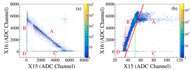
Figure (a) illustrates the energy signal correlation between the adjacent 15th and 16th strips of the DSSD. The plot is divided into four distinct regions:
- Region A: Represents energy-sharing signals between strips.
- Regions B and C: Correspond to induced signals in adjacent strips.
- Region D: Indicates baseline (pedestal) signals.
Figure (b) provides a magnified view of the low-energy end of the horizontal axis in Figure (a). It is observed that as the energy of the 16th strip increases, a small signal is consistently generated on the 15th strip in a fixed proportion. This small signal is referred to as the induced signal from the adjacent strip. The amplitude of the induced signal is proportional to the amplitude of the source signal. When the induced signal’s amplitude falls below the ADC threshold, it is not recorded, resulting in a loss of this signal and a corresponding reduction in multiplicity by 1. This mechanism explains the observed dependence of the energy difference on the amplitude.
Impact Assessment
The maximum observed offset in the data is approximately $40/6000 = 0.006$, which has negligible impact on the physics objectives of the study. Therefore, no further corrections are attempted in subsequent data processing.
Total energy difference cuts
After defining xesc and yesc, the next step is to inspect the correlation between the corrected total energy on one side and the corrected front-back energy difference. In the original ROOT analysis, histograms of the form
$$
xesc \ \text{vs.}\ (xesc-yesc)
$$
are drawn for DSSD1–3, and a graphical cut is placed on the cross-shaped region around the central bright concentration. This cut is loaded from cutd1esc.cut, cutd2esc.cut, and cutd3esc.cut.
gROOT->LoadMacro("cutd1esc.cut");
gROOT->LoadMacro("cutd2esc.cut");
gROOT->LoadMacro("cutd3esc.cut");
c1->Clear();
gStyle->SetOptStat(0);
c1->Divide(3,1);
c1->cd(1);
TCut cdet1 ="x1hit>0 && y1hit>0 ";
tree->Draw("x1esc:x1esc-y1esc>>hds1(200,-100,100,200,0,8000)",cdet1 && "cutd1esc","colz");
gPad->SetLogz();
c1->cd(2);
TCut cdet2 ="x2hit>0 && y2hit>0 ";
tree->Draw("x2esc:x2esc-y2esc>>hds2(200,-100,100,200,0,8000)",cdet2 && "cutd2esc","colz");
gPad->SetLogz();
c1->cd(3);
TCut cdet3 ="x3hit>0 && y3hit>0 ";
tree->Draw("x3esc:x3esc-y3esc>>hds3(200,-100,100,200,0,8000)",cdet3 && "cutd3esc","colz");
gPad->SetLogz();
c1->Draw();
Event Classification
The event classification combines strip multiplicities (xhit, yhit), cluster multiplicities (xm, ym), strip adjacency, and corrected front-back energy matching.
Because a single particle can produce a double-strip response via charge sharing or induced signals, strip multiplicity is not automatically particle multiplicity. Each topology must be examined explicitly.
Notation and Plot Reading
To classify event topologies accurately, we use the following variables and plotting conventions:
- Multiplicities:
xhit/yhitcount fired strips, whilexm/ymcount spatial clusters (adjacent strips merged). Note: Neither automatically equals the true number of incident particles. - Hit Indices:
x[i]andxe[i]are the strip number and raw energy of the $i$-th hit in the event. Adjacency is verified by strip numbers (e.g.,abs(x[0]-x[1]) == 1). - Corrected Energies (Aliases): We subtract empirical offsets (25, 25, 30 for DSSD1, 2, and 3) from the raw energies. In the ROOT code, an alias like
x1ec0represents the energy corrected 0-th hit on the X-side of DSSD1 ($xe[0]-25$). - Reading the Plots: The
tree->Draw("A:B")commands test specific particle-pairing hypotheses by plotting their front-back energy matching errors ($\Delta E$). If a hypothesis is correct, the events will cluster near the origin $(0,0)$.
int off[3] = {25, 25, 30};

// Define energy-corrected (ec) aliases for the first 3 hits in DSSD 1, 2, and 3
for(int id=1; id<=3; id++){
    for(int i=0; i<3; i++){
        tree->SetAlias(Form("x%dec%d", id, i), Form("x%de[%d]-%d", id, i, off[id-1]));
        tree->SetAlias(Form("y%dec%d", id, i), Form("y%de[%d]-%d", id, i, off[id-1]));
    }
}
TCut cut ;
TCanvas *c2 = new TCanvas("c2","c2",900,600);
c2->Clear();
c2->Divide(3,2);
/*
   x: 0 1 |   01  |  0  1  |  01 |
   y: 0 1 |  0  1 |   01   |  01 |
       ——
*/
for(int i=1; i<=3; i++) {
    cut = Form("x%dhit==2 && y%dhit==2 && x%dm==2 && y%dm==2 && cutd%desc",i,i,i,i,i);
    c2->cd(i);
    TString sdraw = Form("x%dec0-y%dec0:x%dec1-y%dec1>>h%da(200,-50,50,200,-50,50)",i,i,i,i,i);
    tree->Draw(sdraw,cut,"colz");
    gPad->SetLogz();
}
/*
   x: 0 1 |   01  |  0  1  |  01 |
   y: 0 1 |  0  1 |   01   |  01 |
               ——
*/
for(int i=1; i<=3; i++) {
    cut = Form("x%dhit==2 && y%dhit==2 && x%dm==1 && y%dm==2 && cutd%desc",i,i,i,i,i);
    c2->cd(i+3);
    TString sdraw = Form("x%dec0-y%dec0:x%dec1-y%dec1>>h%db(200,-50,50,200,-50,50)",i,i,i,i,i);
    tree->Draw(sdraw,cut,"colz");
    gPad->SetLogz();
}

c2->Draw();
TCut cut ;
c2->Clear();
c2->Divide(3,2);
/*
   x: 0 1 |   01  |  0  1  |  01 |
   y: 0 1 |  0  1 |   01   |  01 |
                      ——
*/
for(int i=1; i<=3; i++) {
    cut = Form("x%dhit==2 && y%dhit==2 && x%dm==2 && y%dm==1 && cutd%desc",i,i,i,i,i);
    c2->cd(i);
    TString sdraw = Form("x%dec0-y%dec0:x%dec1-y%dec1>>h%dc(200,-50,50,200,-50,50)",i,i,i,i,i);
    tree->Draw(sdraw,cut,"colz");
    gPad->SetLogz();
}
/*
   x: 0 1 |   01  |  0  1  |  01 |
   y: 0 1 |  0  1 |   01   |  01 |
                              ——
*/
for(int i=1; i<=3; i++) {
    cut = Form("x%dhit==2 && y%dhit==2 && x%dm==1 && y%dm==1 && cutd%desc",i,i,i,i,i);
    c2->cd(i+3);
    TString sdraw = Form("x%dec0-y%dec0:x%dec1-y%dec1>>h%dd(200,-50,50,200,-50,50)",i,i,i,i,i);
    tree->Draw(sdraw,cut,"colz");
    gPad->SetLogz();
}
c2->Draw();
xhit=2 and yhit=3
TCut cut ;
c2->Clear();
c2->Divide(3,2);
/*
x:   0  1 |   0  1  |  0  1 | 01  2 |  0 12  | 02  1  |
y:  01  2 |   0  12 | 02  1 |  0  1 |  0  1  |  0  1  |
      ——
*/

for(int i=1; i<=3; i++) {
    cut = Form("x%dhit==2 && y%dhit==3 && x%dm==2 && y%dm==2 && abs(y%d[0]-y%d[1])==1 && cutd%desc",i,i,i,i,i,i,i);
    c2->cd(i);
    gPad->SetLogz();
    tree->Draw(Form("x%dec0-(y%dec0+y%dec1):x%dec1-y%dec2>>h%da(200,-50,50,200,-50,50)",i,i,i,i,i,i),cut,"colz");;
}
/*
x:   0  1 |   0  1  |  0  1 | 01  2 |  0 12  | 02  1  |
y:  01  2 |   0  12 | 02  1 |  0  1 |  0  1  |  0  1  |
               ——
*/
for(int i=1; i<=3; i++) {
    cut = Form("x%dhit==2 && y%dhit==3 && x%dm==2 && y%dm==2 && abs(y%d[1]-y%d[2])==1 && cutd%desc",i,i,i,i,i,i,i);
    c2->cd(i+3);
    gPad->SetLogz();
    tree->Draw(Form("x%dec0-y%dec0:x%dec1-(y%dec1+y%dec2)>>h%db(200,-50,50,200,-50,50)",i,i,i,i,i,i),cut,"colz");;
}
/*
x:   0  1 |   0  1  |  0  1 | 01  2 |  0 12  | 02  1  |
y:  01  2 |   0  12 | 02  1 |  0  1 |  0  1  |  0  1  |
                        ——
*/
for(int i=1; i<=3; i++) {
    cut = Form("x%dhit==2 && y%dhit==3 && x%dm==2 && y%dm==2 && abs(y%d[0]-y%d[2])==1 && cutd%desc",i,i,i,i,i,i,i);
    c2->cd(i+6);
    gPad->SetLogz();
    tree->Draw(Form("x%dec0-(y%dec0+y%dec2):x%dec1-y%dec1>>h%dc(200,-50,50,200,-50,50)",i,i,i,i,i,i),cut,"colz");;
}

c2->Draw();
xhit=3 and yhit=2
TCut cut ;
TCanvas *c3 = new TCanvas("c3","c3",900,900);
c3->Clear();
c3->Divide(3,3);
/*
x:   0  1 |   0  1  |  0  1 | 01  2 |  0 12  | 02  1  |
y:  01  2 |   0  12 | 02  1 |  0  1 |  0  1  |  0  1  |
                                ——
*/
for(int i=1; i<=3; i++) {
    cut = Form("x%dhit==3 && y%dhit==2 && x%dm==2 && y%dm==2 && abs(x%d[0]-x%d[1])==1 && cutd%desc",i,i,i,i,i,i,i);
    c3->cd(i);
    gPad->SetLogz();
    tree->Draw(Form("(x%dec0+x%dec1)-y%dec0:x%dec2-y%dec1>>h%de(200,-50,50,200,-50,50)",i,i,i,i,i,i),cut,"colz");;
}
/*
x:   0  1 |   0  1  |  0  1 | 01  2 |  0 12  | 02  1  |
y:  01  2 |   0  12 | 02  1 |  0  1 |  0  1  |  0  1  |
                                        ——
*/
for(int i=1; i<=3; i++) {
    cut = Form("x%dhit==3 && y%dhit==2 && x%dm==2 && y%dm==2 && abs(x%d[1]-x%d[2])==1 && cutd%desc",i,i,i,i,i,i,i);
    c3->cd(i+3);
    gPad->SetLogz();
    tree->Draw(Form("x%dec0-y%dec0:(x%dec1+x%dec2)-y%dec1>>h%df(200,-50,50,200,-50,50)",i,i,i,i,i,i),cut,"colz");;
}
/*
x:   0  1 |   0  1  |  0  1 | 01  2 |  0 12  | 02  1  |
y:  01  2 |   0  12 | 02  1 |  0  1 |  0  1  |  0  1  |
                                                 ——
*/
for(int i=1; i<=3; i++) {
    cut = Form("x%dhit==3 && y%dhit==2 && x%dm==2 && y%dm==2 && abs(x%d[0]-x%d[2])==1 && cutd%desc",i,i,i,i,i,i,i);
    c3->cd(i+6);
    gPad->SetLogz();
    tree->Draw(Form("(x%dec0+x%dec2-y%dec0):x%dec1-y%dec1>>h%dg(200,-50,50,200,-50,50)",i,i,i,i,i,i),cut,"colz");;
}
c3->Draw();
TCut cut ;
c3->Clear();
c3->Divide(3,3);
for(int i=1; i<=3; i++) {
    cut = Form("x%dhit==3 && y%dhit==3 && x%dm==3 && y%dm==3 && cutd%desc",i,i,i,i,i);
    c3->cd(3*i-2);
    gPad->SetLogz();
    tree->Draw(Form("x%dec0-y%dec0:x%dec1-y%dec1>>h%da(200,-50,50,200,-50,50)",i,i,i,i,i),cut ,"colz");
    c3->cd(3*i-1);
    gPad->SetLogz();
    tree->Draw(Form("x%dec0-y%dec0:x%dec2-y%dec2>>h%db(200,-50,50,200,-50,50)",i,i,i,i,i),cut ,"colz");
    c3->cd(3*i);
    gPad->SetLogz();
    tree->Draw(Form("x%dec1-y%dec1:x%dec2-y%dec2>>h%dc(200,-50,50,200,-50,50)",i,i,i,i,i),cut ,"colz");
}
c3->Draw();
Assignment
Note: Multiple particles may be incident on the same strip, for example, two particles at coordinates (16,14) and (16,15). In such cases, the amplitude relationship is given by $A'_{x16} = A'_{y14} + A'_{y15}$.
1. For the topology xhit=3 and yhit=3:
- Determine the energy-matching conditions for other possible three-particle configurations (i.e., different permutations of x-y pairings).
- Determine the conditions for all possible two-particle configurations within this topology (e.g., when adjacent strips are fired by a single particle).
- Provide the corresponding ROOT plots to verify your conditions.
2. For the asymmetric topologies xhit=2 and yhit=3 (or xhit=3 and yhit=2):
- Determine the energy-matching conditions for a three-particle event. (Hint: Apply the shared-strip logic described in the Note above).
- Provide the corresponding ROOT plots to verify your conditions.
3. Based on the event classification logic discussed in this section, write a ROOT macro to fully reconstruct the events.
- Determine the true number of incident particles (
hit) for each detector based on your topology tests. - Assign the final particle energy
eusing the corrected x-side energy. - Save the reconstructed events into a new ROOT file (e.g.,
evt_16C.root) using the following tree structure:
// det1
Int_t  hit1;
double e1[hit1];
Int_t  x1[hit1], y1[hit1];

// det2
Int_t  hit2;
double e2[hit2];
Int_t  x2[hit2], y2[hit2];  // Note: fixed the index typo here

// det3
Int_t  hit3;
double e3[hit3];
Int_t  x3[hit3], y3[hit3];