3.5 DSSD front-back Correlation(II) - dssd1

Purpose:

  • Based on the x-y correlation, normalize the amplitudes of all strips using the amplitude of a given strip as a reference.

Normalization

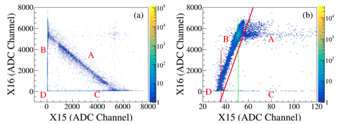
  • For a particle depositing energy $E$ at the intersection $(x_i, y_j)$ in a DSSD, the raw signal amplitudes $a_{xi}$ (from front strip $x_i$) and $a_{yj}$ (from back strip $y_j$) satisfy a linear relationship: $$ a_{xi} = k_{yj} a_{yj} + b_{yj}, $$ where $k_{yj}$ and $b_{yj}$ are normalization coefficients derived from energy calibration.

  • The goal is to normalize the amplitudes of all x- and y-strips relative to a reference strip (e.g., $x_i$) to ensure a consistent energy scale across the detector. This involves determining linear coefficients that align each strip’s amplitude to the reference.

Method 1: Pixel Normalization

  1. Select a Reference Strip: Fix $x_i^*$ as the reference strip. For each y-strip $y_j$ ($j = 0, 1, \dots, N_y$), use the linear relationship:

    $$ a_{xi^*} = k_{yj} a_{yj} + b_{yj}, $$

    to obtain normalization coefficients $\{ k_{yj}, b_{yj} \}$ by fitting events at the $(x_i, y_j)$ pixel. Sufficient event statistics are required for each pixel.

  2. Normalize Y-Strips: Apply the coefficients to normalize all y-strip amplitudes:

    $$ a_{yj}' = k_{yj} a_{yj} + b_{yj}, \quad j = 0, 1, \dots, N_y. $$
  3. Normalize X-Strips: Select a normalized y-strip (e.g., $y_j^*$) as the new reference. For each x-strip $x_k$ ($k = 0, 1, \dots, N_x$), fit:

    $$ a'_{yj*} = k_{xk} a_{xk} + b_{xk}, $$

    to obtain coefficients $\{ k_{xk}, b_{xk} \}$ and normalize x-strip amplitudes:

    $$ a'_{xk} = k_{xk} a_{xk} + b_{xk}. $$

After these steps, all x- and y-strip amplitudes are normalized to the energy scale of the initial reference strip $x_i$. This method relies on sufficient event statistics at each $(x_i, y_j)$ pixel for accurate fitting.

Method 2: Strip Normalization

This method normalizes a DSSD by starting with the strips that detect the most particles and gradually normalizing others, ensuring all strips measure energy consistently.

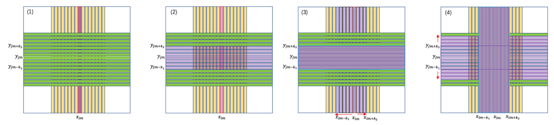
  1. Identify High-Statistics Strips: Select the x-strip $x_{i^*}$ or y-strip $y_{j^*}$ with the highest event counts, typically in the detector’s central or most active regions.

  2. Normalize Back Strips: Use $x_{i^*}$ as the reference to normalize nearby back strips $y_j$ (those close to $y_{j^*}$ with enough hits). For each $y_j$, fit the relationship:

    $$ a_{x_{i^*}} = k_{yj} a_{yj} + b_{yj}, $$

    to find coefficients $k_{yj}$ and $b_{yj}$. Then normalize the back strip signals:

    $$ a'_{yj} = k_{yj} a_{yj} + b_{yj}. $$
  3. Normalize Front Strips: Group the normalized back strips (from $y_j$ near $y_{j^*}$) into a single reference $y_{js}'$, like a wider strip. Use this to normalize nearby front strips $x_i$ (those close to $x_{i^*}$ with enough hits). For each $x_i$, fit:

    $$ a'_{yj_s} = k_{xi} a_{xi} + b_{xi}, $$

    to find coefficients $k_{xi}$ and $b_{xi}$. Then normalize the front strip signals:

    $$ a'_{xi} = k_{xi} a_{xi} + b_{xi}. $$
  4. Spread Outward: Repeat the process, using newly normalized front or back strips as references to normalize strips farther out. Continue until all strips are normalized, ensuring enough particle hits for accurate fitting at each step.

图片名称

DSSD1 Normalization

The following analysis, using DSSD1 as an example, applies Method 2 to normalize amplitudes using coefficients $k_{yj}$ and $b_{yj}$ for y-strips and $k_{xi}$ and $b_{xi}$ for x-strips, achieving a consistent energy scale across strips.

In [1]:
//%jsroot on
TCanvas *c1 = new TCanvas("c1","c1");
TFile *fin = new TFile("./data/d1xy.root");
TTree *tree =(TTree *)fin->Get("tree");
c1->SetLogz();
In [2]:
tree->Draw("ye:xe>>(8000,0,8000,8000,0,8000)","","colz");
c1->Draw();

Reference Strip Selection

The x-direction strip at ix=16 has the highest statistics, so it is chosen as the reference strip.

  • For ix=16, the y-direction strips iy=8 to iy=16 have statistics exceeding 600 counts.

The first step is to use the x-strip amplitude xe[16] as the reference to fit the y-strip amplitudes ye[iy] for iy=8 to iy=16, obtaining the normalization coefficients for the y-direction.

In [3]:
tree->Draw("iy:ix>>hxy(32,0,32,32,0,32)","","colz");
c1->Draw();
In [4]:
tree->Draw("iy>>hy(32,0,32)","","goff");
tree->Draw("ix>>hx(32,0,32)","","goff");
auto hx=(TH1F*)gROOT->FindObject("hx");
auto hy=(TH1F*)gROOT->FindObject("hy");
hx->Draw();
hy->Draw("same");
hy->SetLineColor(kRed);
c1->Draw();
In [5]:
tree->Draw("iy>>hy2(32,0,32)","ix==16","colz");
c1->Draw();

Note

  • The figure below shows that data points are excessively concentrated around 400-700 channels, which leads to an overemphasis on the weights of low-energy points during fitting.

  • To balance fitting accuracy across different regions of the dynamic range, it is sometimes necessary to reduce the density of points in regions with excessively high weights.

In [6]:
c1->Clear();
tree->Draw("xe>>hxe(100,0,1000)","","goff");
tree->Draw("ye>>hye(100,0,1000)","","goff");
auto hxe=(TH1F*)gROOT->FindObject("hxe");
auto hye=(TH1F*)gROOT->FindObject("hye");
hxe->Draw();
hye->Draw("same");
hye->SetLineColor(kRed);
c1->SetLogy();
gPad->SetGrid(1,1);
c1->Draw();
c1->SetLogy(0);

TTree events

In [7]:
// Open input file and get TTree
TFile *fin = new TFile("./data/d1xy.root");
TTree *tree = (TTree*)fin->Get("tree");

// Set branch addresses
Int_t ix, iy;
Int_t xe, ye; // Raw amplitudes (a_xi, a_yj)
tree->SetBranchAddress("ix", &ix);
tree->SetBranchAddress("iy", &iy);
tree->SetBranchAddress("xe", &xe); 
tree->SetBranchAddress("ye", &ye);

Fitting

In [8]:
double parx[32][3], pary[32][3]; //global 
for(int i=0; i<32; i++) {
    parx[i][0] = 0.;  parx[i][1] = 1.; parx[i][2] = 0.;
    pary[i][0] = 0.;  pary[i][1] = 1.; pary[i][2] = 0.;
}
TCanvas *c_all = new TCanvas("c_all","c_all", 800,1200);

Fitting Function

Functionality:

  • fitmethod="fitx":

    • Normalize x-strip amplitudes (xe) in the range ix1 to ix2 using known normalization coefficients (parx[ix][0:2]).

    • Uses the normalized x-strip amplitudes as a reference to calibrate y-strip amplitudes (ye) in the range iy1 to iy2.

    • Stores the resulting normalization coefficients in the pary array for y-strips.

  • fitmethod="fity":

    • Normalizes y-strip amplitudes (ye) in the range iy1 to iy2 using known normalization coefficients (pary[iy][0:2]).

    • Uses the normalized y-strip amplitudes as a reference to normalize x-strip amplitudes (xe) in the range ix1 to ix2.

    • Stores the resulting normalization coefficients in the parx array for x-strips.

Output:

  • Saves histograms as PNG files (e.g., fity{id}.png or fitx{id}.png), overwriting any existing files to retain only the latest results.

  • Prints a table with fit parameters (p0, p1, p2), reduced chi-square (chi2/ndf), amplitude ranges (ymin, ymax), and point counts (Ncounts) for each fitted strip.

In [9]:
void fit(Int_t ix1, Int_t ix2, Int_t iy1, Int_t iy2, TString fitmethod)
{
    // Validate input ranges
    if (ix1 > ix2 || iy1 > iy2 || ix1 < 0 || ix2 >= 32 || iy1 < 0 || iy2 >= 32) {
        printf("Error: Invalid strip ranges (ix1=%d, ix2=%d, iy1=%d, iy2=%d)\n", ix1, ix2, iy1, iy2);
        return;
    }

    // Set strip range and identifier based on fitmethod
    int id1 = ix1;
    int id2 = ix2;
    TString sid = "ix";
    if (fitmethod == "fity") {
        id1 = iy1;
        id2 = iy2;
        sid = "iy";
    }

    // Create TGraph and TH2F arrays for each strip
    TGraph *gc[32];
    TH2F *h2res[32]; // Residual plots
    Int_t ngc[32];   // Number of points per graph
    for (Int_t i = 0; i < 32; i++) {
        gc[i] = new TGraph();
        h2res[i] = new TH2F(Form("h2res%s%2d", sid.Data(), i),
                            Form("Residuals %s-strip %d;Residual;Amplitude", sid.Data(), i),
                            100, -50, 50, 800, 0, 8000);
        ngc[i] = 0;
    }

    // Read TTree entries
    Long64_t nentries = tree->GetEntries();
    for (Long64_t jentry = 0; jentry < nentries; jentry++) {
        tree->GetEntry(jentry);

        // Include only events within specified strip ranges
        if (ix < ix1 || ix > ix2 || iy < iy1 || iy > iy2) continue;

        if (fitmethod == "fity") {
            double e = parx[ix][0] + xe * parx[ix][1] + xe * xe * parx[ix][2]; // Calibrated x-strip amplitude
            
           // Downsample points around 500 channels (optional, based on prior note)
            if (TMath::Abs(ye - 500) < 100 && gRandom->Rndm() > 0.2) continue;
            
            gc[iy]->SetPoint(ngc[iy]++, ye, e);
        } else {
            double e = pary[iy][0] + ye * pary[iy][1] + ye * ye * pary[iy][2]; // Calibrated y-strip amplitude
            
            // Downsample points around 500 channels (optional, based on prior note)
            if (TMath::Abs(ye - 500) < 100 && gRandom->Rndm() > 0.2) continue;
            
            gc[ix]->SetPoint(ngc[ix]++, xe, e);
        }
        if (jentry % 10000 == 0) cout << ".";
    }
    cout << endl;
    
    double par[32][3],c2n[32];    
    for(int i=0; i<32; i++) {
        par[i][0] = 0.;  par[i][1] = 1.; par[i][2] = 0.; 
        c2n[i] = -1;
    }
    // Print header for console output
    cout << Form("%4s%9s%10s%15s%14s%5s%7s%10s", sid.Data(), "p0", "p1", "p2", "chi2/ndf", "ymin", "ymax", "Ncounts") << endl;

    // Fit graphs and update parameters
    for (Int_t id = id1; id <= id2; id++) {
        if (ngc[id] < 20) {
            printf("Warning: Too few points (%d) for %s-strip %d\n", ngc[id], sid.Data(), id);
            continue;
        }

        // Fit with pol2 using robust fitting
        gc[id]->Fit("pol2", "Q ROB");
        TF1 *fit = gc[id]->GetFunction("pol2");
        if (!fit) {
            printf("Error: Fit failed for %s-strip %d\n", sid.Data(), id);
            for (int i = 0; i < 3; i++) par[id][i] = (i == 1) ? 1.0 : 0.0; // Default: p1=1, p0=p2=0
            c2n[id] = 0.0;
            continue;
        }

        // Store fit parameters
        for (int i = 0; i < 3; i++) {
            par[id][i] = fit->GetParameter(i);
        }
        c2n[id] = (fit->GetNDF() > 0) ? fit->GetChisquare() / fit->GetNDF() : 0.0;

        // Fill residual histogram
        double *x = gc[id]->GetX();
        double *y = gc[id]->GetY();
        for (Int_t i = 0; i < gc[id]->GetN(); i++) {
            h2res[id]->Fill(y[i] - (par[id][0] + x[i] * par[id][1] + x[i] * x[i] * par[id][2]), x[i]);
        }

        // Compute data range for output
        Double_t xmin, xmax, ymin, ymax;
        gc[id]->ComputeRange(xmin, ymin, xmax, ymax);

        // Print fit results
        cout << Form("%4d%9.2f%10.6f%15e%12.2f%7d%7d%8d",
                     id, par[id][0], par[id][1], par[id][2], c2n[id], int(xmin), int(xmax), ngc[id]) << endl;
    }
        // Suppress TCanvas::Print info messages
    Int_t oldIgnoreLevel = gErrorIgnoreLevel;
    gErrorIgnoreLevel = kWarning; 
    
    c_all->Clear();
    // Display all histograms in a single canvas
    c_all->SetName(Form("c_all_%s", fitmethod.Data()));
    c_all->SetTitle(Form("Residuals for %s", fitmethod.Data()));
    c_all->Divide(4, 8); // 4x grid for up to 32 strips
    for (Int_t id = 0; id < 32; id++) {
        if (id >= id1 && id <= id2 && ngc[id] >= 3) {
            c_all->cd(id + 1);
            h2res[id]->Draw("colz");
        }
    }
    c_all->Update();
    c_all->SaveAs(Form("all_residuals_%s.png", fitmethod.Data())); // Save combined plot, overwriting previous

    // Optionally save individual histograms (if desired)
    for (Int_t id = id1; id <= id2; id++) {
        if (ngc[id] < 3) continue;
        TCanvas *c_single = new TCanvas();
        h2res[id]->Draw("colz");
        c_single->SaveAs(Form("%s%2d.png", fitmethod.Data(), id)); // Overwrites individual plots
        delete c_single;
    }

    // Update calibration parameters
    for (Int_t i = 0; i < 32; i++) {
        for (Int_t id = 0; id < 3; id++) {
            if (fitmethod == "fity") {
                pary[i][id] = par[i][id];
            } else {
                parx[i][id] = par[i][id];
            }
        }
    }

    // Clean up
    for (Int_t i = 0; i < 32; i++) {
        delete gc[i];
        delete h2res[i];
    }
}
In [10]:
void viewFit(TString cfit="fity") {
    // Load TImage
    TImage *img = TImage::Open(Form("all_residuals_%s.png",cfit.Data()));
    if (!img || !img->IsValid()) {
        printf("Error: Cannot open or invalid image file\n");
        return;
    }
    c_all->Clear();
    // Create TCanvas
    img->Draw("xxx"); // Draw image, scaling to fit canvas
    c_all->Draw();
}
In [11]:
fit(16,16,8,16,"fity");//normalize iy=8-16 using ix=16 as a reference.
viewFit("fity");
  iy       p0        p1             p2      chi2/ndf ymin   ymax   Ncounts
   8     6.34  0.995782  -6.022345e-07     3485.83    206   7192     485
   9     9.33  0.966250  -4.694504e-07     3103.46    204   7435     505
  10    10.81  0.990107  -3.594162e-07     3207.99    203   7618     510
  11    13.31  0.985029  -5.749746e-07     4343.34    207   7133     531
  12    11.45  1.002328  -4.272509e-07     4982.98    202   7478     588
  13    13.26  0.982740  -4.872860e-07     3544.32    206   7331     529
  14     7.30  0.982585  -3.471350e-07     3009.33    206   7591     498
  15    15.73  0.991847  -6.140406e-07     3458.56    209   6939     495
  16    -3.67  0.981624  -1.354263e-07     2564.52    205   7267     497

Determining the Next Fitting Range for ix

  • After combining iy=8 to 16, all x-strips (ix) have statistics exceeding 800 counts. The next step is to fit the entire ix range.
In [12]:
c1->Clear();
tree->Draw("ix>>hx2(32,0,32)","iy>=8 && iy<=16","colz");
c1->Draw();

Combine ye[iy] for iy=8 to 16 and Normalize All X-Direction Strips

  • ix=16 is the reference strip for normalization. The parameters fitted for ix=16 should satisfy p0 ≈ 0 and p1 ≈ 1.
In [13]:
fit(0,31,8,16,"fitx");//Normalize ix=0-31 using iy=8-16 as a reference.
viewFit("fitx");
....
  ix       p0        p1             p2      chi2/ndf ymin   ymax   Ncounts
   0     8.46  1.003254  -4.092288e-07     5924.04    203   5048     462
   1     3.29  1.009565  -1.281270e-07     4051.10    201   6044     601
   2    -1.37  1.010772  -1.493311e-07     4403.92    204   6279     765
   3     3.59  0.993332  -1.272292e-07     4567.71    203   5561     963
   4    -0.87  1.002187   5.116375e-08     4172.80    202   5776    1159
   5     4.31  1.020447  -1.372421e-07     3940.21    202   5779    1214
   6    -0.31  1.015887  -1.803111e-07     3739.98    201   7131    1368
   7     4.06  1.012642  -1.918537e-07     4117.16    203   6065    1474
   8    -0.36  1.009654   4.398601e-08     3936.28    204   6490    1593
   9     5.74  1.006721   5.786466e-08     4334.29    204   6550    1739
  10     1.80  1.023363  -7.141691e-08     3749.34    203   6533    1898
  11     5.61  1.017001   1.505519e-08     4175.00    202   6494    1991
  12     1.56  0.995778   5.832561e-08     4685.25    206   6999    2180
  13     5.69  1.021925  -1.398511e-07     4381.35    201   6552    2285
  14    -0.52  1.028060  -1.710230e-09     3783.71    207   7028    2605
  15     8.61  1.002989  -2.714062e-09     4442.84    202   7188    3115
  16    -0.13  1.000071  -8.394350e-09     3568.91    201   7532    4650
  17     6.18  1.006740  -1.103175e-07     3656.23    202   6853    3752
  18    -0.57  1.014407  -1.935309e-08     3518.66    201   7059    3880
  19     2.74  0.982565  -7.532754e-08     3949.72    201   7252    3705
  20    -1.43  1.012154  -7.432916e-08     3390.44    201   6883    3461
  21     2.30  1.010532  -1.356765e-07     3537.28    201   6396    2671
  22    -1.78  1.002057  -9.575259e-08     3407.13    204   6830    2487
  23     4.90  1.007365  -1.415383e-07     3664.97    205   6837    2225
  24     1.97  0.990699  -1.215343e-08     3122.05    204   6802    1985
  25     1.18  0.979550  -2.657120e-08     4436.40    204   5999    1677
  26    -0.15  0.986241   2.291745e-08     4324.03    201   5218    1446
  27     1.89  0.974479  -1.413247e-07     4229.90    202   6012    1360
  28     0.13  0.966676   4.083955e-08     4326.20    201   5597    1087
  29    -0.54  1.001352  -1.865900e-07     4317.67    201   5724     905
  30     1.03  1.005603  -1.147835e-07     4758.06    211   5110     649
  31     1.80  0.970394  -1.213873e-07     6631.23    201   5873     568

Combine xe[ix] for ix=0 to 31 and normalize All y-Direction Strips

In [14]:
fit(0,31,0,31,"fity");//normalize iy=0-31 using ix=0-31 as a reference.
viewFit("fity");
...............
  iy       p0        p1             p2      chi2/ndf ymin   ymax   Ncounts
   0    21.32  0.957864  -3.387427e-07     5088.88    201   6619    2114
   1    14.73  0.977752  -5.082355e-07     4485.38    201   6842    2765
   2    14.68  0.972536  -2.477686e-07     3959.65    201   6742    3466
   3    19.06  0.978160  -5.540858e-07     4170.28    201   7594    4151
   4     6.76  0.979623  -2.980852e-07     3613.70    201   7007    4749
   5    14.04  0.988459  -4.429188e-07     4191.46    201   7393    5101
   6     8.46  0.984455  -3.913559e-07     3648.55    201   7481    5575
   7    17.17  0.995673  -6.826582e-07     4206.71    201   7037    5968
   8     6.82  0.995167  -4.845390e-07     3858.06    201   7192    6564
   9     9.70  0.966163  -4.719916e-07     3783.79    201   7435    6834
  10    10.37  0.990608  -4.398066e-07     4171.52    201   7618    6976
  11    13.33  0.984884  -5.344085e-07     4098.80    201   7370    6957
  12    11.61  1.002316  -4.322083e-07     4456.03    201   7478    7256
  13    13.49  0.982738  -4.883047e-07     3734.06    201   7331    7002
  14     6.74  0.982853  -3.892135e-07     3783.86    202   7591    7155
  15    16.19  0.991377  -5.519719e-07     4219.83    201   7294    6502
  16    -3.82  0.981550  -1.181934e-07     3543.12    201   7306    6526
  17    10.06  0.971308  -2.381828e-07     3633.85    201   7543    6192
  18    -0.42  1.002069  -2.437541e-07     4137.49    201   7192    5758
  19     6.58  0.998503  -3.168390e-07     3981.47    201   6912    5170
  20   -10.24  0.983113  -1.037350e-07     3469.68    201   6914    4958
  21     1.86  0.968452  -1.265026e-07     4748.42    202   7086    5275
Warning: Too few points (0) for iy-strip 22
  23     4.64  0.958338  -4.395598e-07     5108.39    201   7376    4940
  24     3.80  0.993235  -1.421546e-07     3738.96    201   6884    3510
  25    -1.63  0.976145  -2.634079e-07     3721.12    203   5962    3488
  26    -1.34  0.994806  -1.159809e-07     3971.75    202   6264    3084
  27     7.11  0.983336  -2.885836e-07     3771.64    201   6073    2640
  28    -4.47  0.983723   3.934468e-07     4101.90    208   6005    2163
  29    -3.11  0.968889   3.304730e-07     4215.45    209   6566    1751
  30    -0.97  0.978872  -4.897855e-07     4493.97    203   5508    1218
  31     0.74  0.970294  -2.144467e-07     5332.04    206   6423    1137

Save normalization factors

In [15]:
void saveParameters(const char* filename = "normalization_parameters.txt") {
    // Open output file (overwrite mode)
    std::ofstream outFile(filename, std::ios::out);
    if (!outFile.is_open()) {
        printf("Error: Cannot open %s for writing\n", filename);
        return;
    }

    // Header
    outFile << "Normalization Parameters\n";
    outFile << "---------------------\n";

    // X-strip parameters (parx)
    outFile << "X-strips (ix):\n";
    outFile << Form("%4s%9s%10s%15s\n", "ix", "p0", "p1", "p2");
    for (Int_t id = 0; id < 32; id++) {
        outFile << Form("%4d%9.2f%10.6f%15e\n",
                        id, parx[id][0], parx[id][1], parx[id][2]);
    }

    // Y-strip parameters (pary)
    outFile << "\nY-strips (iy):\n";
    outFile << Form("%4s%9s%10s%15s\n", "iy", "p0", "p1", "p2");
    for (Int_t id = 0; id < 32; id++) {
        outFile << Form("%4d%9.2f%10.6f%15e\n",
                        id, pary[id][0], pary[id][1], pary[id][2]);
    }

    outFile << "---------------------\n";
    outFile.close();
}
In [16]:
saveParameters("cal_dssd1.txt");

Read Parameters

Double_t parx[32][3], pary[32][3];
readParameters("normalization_parameters.txt", parx, pary);
In [17]:
void readParameters(const char* filename, Double_t (&parx)[32][3], Double_t (&pary)[32][3]) {
    // Open input file
    std::ifstream inFile(filename);
    if (!inFile.is_open()) {
        printf("Error: Cannot open %s\n", filename);
        return;
    }

    // Skip header lines (first 4 lines: title, separator, X-strips header, column labels)
    std::string line;
    for (int i = 0; i < 4; i++) {
        std::getline(inFile, line);
    }

    // Read x-strip parameters (32 lines)
    for (int id = 0; id < 32; id++) {
        int read_id;
        double p0, p1, p2;
        inFile >> read_id >> p0 >> p1 >> p2;

        if (!inFile.good() || read_id != id) {
            printf("Error: Invalid x-strip data at id=%d\n", id);
            inFile.close();
            return;
        }
        parx[id][0] = p0;
        parx[id][1] = p1;
        parx[id][2] = p2;
    }

    // Skip y-strip header lines (2 lines: blank, Y-strips header, column labels)
    for (int i = 0; i < 4; i++) {
        std::getline(inFile, line);
    }

    // Read y-strip parameters (32 lines)
    for (int id = 0; id < 32; id++) {
        int read_id;
        double p0, p1, p2;
        inFile >> read_id >> p0 >> p1 >> p2;

        if (!inFile.good() || read_id != id) {
            printf("Error: Invalid y-strip data at id=%d\n", id);
            inFile.close();
            return;
        }
        pary[id][0] = p0;
        pary[id][1] = p1;
        pary[id][2] = p2;
    }

    inFile.close();
    printf("Read parameters from %s\n", filename);
}
In [18]:
TCanvas *c_plots = new TCanvas("c_plots", "Calibrated Plots", 1200, 600);

// Create histograms
TH2F *h_xy = new TH2F("h_xy", "Normalize xe vs ye;xe (keV);ye (keV)",
                      4000, 0, 8000, 4000, 0, 8000);
TH2F *h_xdiff = new TH2F("h_xdiff", "Calibrated xe vs ye-xe;xe (keV);ye-xe (keV)",
                         100, -50, 50, 4000, 0, 8000);
In [19]:
void calibrateAndPlot(const char* paramFile = "calibration_parameters.txt") {
    
    Double_t parx[32][3], pary[32][3]; //
    
    // Read normalization parameters
    readParameters(paramFile, parx, pary);

    h_xy->Clear();
    h_xdiff->Clear();
    // Loop over TTree entries to calibrate xe, ye
    Long64_t nentries = tree->GetEntries();
    for (Long64_t jentry = 0; jentry < nentries; jentry++) {
        tree->GetEntry(jentry);

        // Validate strip indices
        if (ix < 0 || ix >= 32 || iy < 0 || iy >= 32) continue;

        // Calibrate xe and ye
        Double_t cxe = parx[ix][0] + xe * parx[ix][1] + xe * xe * parx[ix][2];
        Double_t cye = pary[iy][0] + ye * pary[iy][1] + ye * ye * pary[iy][2];

        // Fill histograms
        h_xy->Fill(cxe, cye);
        h_xdiff->Fill(cye - cxe, cxe);

        if (jentry % 10000 == 0) cout << ".";
    }
    cout << endl;

    c_plots->Clear();
    c_plots->Divide(2, 1);

    // Draw xe:ye plot
    c_plots->cd(1);
    h_xy->Draw("colz");

    // Draw xe:ye-xe plot
    c_plots->cd(2);
    h_xdiff->Draw("colz");

    c_plots->Update();
 
}

Check the X-Y correlation and residual plot after normalization

In [20]:
calibrateAndPlot("cal_dssd1.txt");
c_plots->SetLogz();
c_plots->Draw();
Read parameters from cal_dssd1.txt
......................

Front-back energy normalization on DSSD1, DSSD2, and DSSD3.

- Record the normalized events in a structured hit format.
  - For each detector, sort the front and back signals in descending order of amplitude.
  - Detection threshold: Set to 100 channels (discard signals below this value).

Output File Event Structure

Int_t  x1hit;      //multiplicity
Int_t  x1[x1hit];  //Strip 
double  x1e[x1hit]; //energy

Int_t  y1hit;
Int_t  y1[y1hit];
Int_t  y1e[y1hit];

double x1es,y1es; //total energy of x,y side.
int x1m,y1m;      //multiplicity, adjacent tracks are counted as one.
...

ROOT file: cal_16C.root

Offset Correction

In [21]:
TFile *ipf = new TFile("./data/cal_16C.root");
TTree *tree = (TTree*)ipf->Get("tree");

x-y correlation

In [22]:
c1->Clear();
c1->SetWindowSize(1200,300);
c1->Divide(3,1);
c1->cd(1);
tree->Draw("x1es:y1es>>hs1(200,0,10000,200,0,10000)","x1hit>0 && y1hit>0","colz");
gPad->SetLogz();
c1->cd(2);
tree->Draw("x2es:y2es>>hs2(200,0,10000,200,0,10000)","x2hit>0 && y2hit>0","colz");
gPad->SetLogz();
c1->cd(3);
tree->Draw("x3es:y3es>>hs3(200,0,10000,200,0,10000)","x3hit>0 && y3hit>0","colz");
gPad->SetLogz();
c1->Draw();

Hit Pattern

In [23]:
c1->Clear();
c1->SetWindowSize(1200,300);
c1->Divide(3,1);
c1->cd(1);
gPad->SetLogz();
tree->Draw("x1hit:y1hit>>ha(4,1,5,4,1,5)","","colz");
c1->cd(2);
gPad->SetLogz();
tree->Draw("x2hit:y2hit>>hb(4,1,5,4,1,5)","","colz");
c1->cd(3);
gPad->SetLogz();
tree->Draw("x3hit:y3hit>>hc(4,1,5,4,1,5)","","colz");
c1->Draw();

Difference in total energy between the X and Y sides

  • The energy difference between the two sides is not always centered at zero. Instead, it clusters around several specific offset values, with equal spacing between adjacent offsets.
In [24]:
TCut cdet1 ="x1hit>0 && y1hit>0 ";
TCut cdet2 ="x2hit>0 && y2hit>0";
TCut cdet3 ="x3hit>0 && y3hit>0";
c1->Clear();
c1->SetWindowSize(1200,400);
gStyle->SetOptStat(0);
c1->Divide(3,1);
c1->cd(1);
tree->Draw("x1es:x1es-y1es>>hds1(200,-100,100,200,0,8000)",cdet1,"colz");
gPad->SetLogz();
c1->cd(2);
tree->Draw("x2es:x2es-y2es>>hds2(200,-100,100,200,0,8000)",cdet2,"colz");
gPad->SetLogz();
c1->cd(3);
tree->Draw("x3es:x3es-y3es>>hds3(200,-100,100,200,0,8000)",cdet3,"colz");
gPad->SetLogz();
c1->Draw();

total energy difference vs. multiplicity difference

  • The energy difference between the two sides shows linear dependence on the multiplicity difference.
In [25]:
c1->Clear();
c1->SetWindowSize(1200,300);
gStyle->SetOptStat(0);
c1->Divide(3,1);
c1->cd(1);
tree->Draw("x1hit-y1hit:x1es-y1es>>h2ds1(50,-100,100,6,-3,3)",cdet1 ,"colz");
gPad->SetLogz();
c1->cd(2);
tree->Draw("x2hit-y2hit:x2es-y2es>>h2ds2(50,-100,100,6,-3,3)",cdet2,"colz");
gPad->SetLogz();
c1->cd(3);
tree->Draw("x3hit-y3hit:x3es-y3es>>h2ds3(50,-100,100,6,-3,3)",cdet3,"colz");
gPad->SetLogz();
c1->Draw();

Correction

After normalization, the amplitude $A'_i$ of each strip satisfies the linear relationship $E_i = k A'_i + b$, where $E_i$ is the energy. Let the multiplicity of the x-side be $m_x$ and the y-side be $m_y$. The normalized amplitude sums for the x-side and y-side are defined as:

$$ x1es = \sum_{{i}\in m_x} A'_{xi}, \quad y1es = \sum_{{j}\in m_y} A'_{yj} $$

The total energies for the x-side and y-side are then:

$$ \begin{align} E_x = k \cdot x1es + m_x b \\ E_y = k \cdot y1es + m_y b \end{align} $$

Assuming energy conservation ($E_x = E_y$), the difference in amplitude sums is:

$$ x1es - y1es = (m_y - m_x) \frac{b}{k} $$
  • Case 1: Equal Multiplicities ($m_x = m_y$)

    • The amplitude difference is zero: $x1es - y1es = 0$.
  • Case 2: Unequal Multiplicities ($m_x \neq m_y$)

    • The amplitude difference is non-zero.
    • The larger the multiplicity difference $m_y - m_x$, the greater the value of the difference.
    • The sign of the difference depends on the sign of $b$.
    • From the figure above, it is evident that for DSSD1, DSSD2, and DSSD3, the ratio $b/k$ is approximately 25, 25 and 30, respectively.

Offset corrected amplitude:$A''=A'-b/k$ $$ \begin{align} E_x = k \cdot x1es' \\ E_y = k \cdot y1es' \end{align} $$ namely, $$ x1es' - y1es' = 0 $$

In [26]:
c1->Clear();
c1->SetWindowSize(1200,400);
gStyle->SetOptStat(0);
c1->Divide(3,1);
c1->cd(1);
TCut cdet1 ="x1hit>0 && y1hit>0 ";
tree->SetAlias("x1esc","x1es+x1hit*(-25)");
tree->SetAlias("y1esc","y1es+y1hit*(-25)");
tree->Draw("x1esc:x1esc-y1esc>>hds1(200,-100,100,200,0,8000)",cdet1,"colz");
gPad->SetLogz();
c1->cd(2);
TCut cdet2 ="x2hit>0 && y2hit>0 ";
tree->SetAlias("x2esc","x2es+x2hit*(-25)");
tree->SetAlias("y2esc","y2es+y2hit*(-25)");
tree->Draw("x2esc:x2esc-y2esc>>hds2(200,-100,100,200,0,8000)",cdet2,"colz");
gPad->SetLogz();
c1->cd(3);
TCut cdet3 ="x3hit>0 && y3hit>0 ";
tree->SetAlias("x3esc","x3es+x3hit*(-30)");
tree->SetAlias("y3esc","y3es+y3hit*(-30)");
tree->Draw("x3esc:x3esc-y3esc>>hds3(200,-100,100,200,0,8000)",cdet3,"colz");
gPad->SetLogz();
c1->Draw();

Adjacent Strip Effects

After applying the correction by subtracting the corresponding $b/k$ value from each strip’s amplitude, the energy difference between the x-side and y-side still exhibits a dependence on the amplitude of one side. This is attributed to induced signals between adjacent strips.

Detailed Correlation Between Adjacent Strips

Figure (a) illustrates the energy signal correlation between the adjacent 15th and 16th strips of the DSSD. The plot is divided into four distinct regions:

  • Region A: Represents energy-sharing signals between strips.
  • Regions B and C: Correspond to induced signals in adjacent strips.
  • Region D: Indicates baseline (pedestal) signals.

Figure (b) provides a magnified view of the low-energy end of the horizontal axis in Figure (a). It is observed that as the energy of the 16th strip increases, a small signal is consistently generated on the 15th strip in a fixed proportion. This small signal is referred to as the induced signal from the adjacent strip. The amplitude of the induced signal is proportional to the amplitude of the source signal. When the induced signal’s amplitude falls below the ADC threshold, it is not recorded, resulting in a loss of this signal and a corresponding reduction in multiplicity by 1. This mechanism explains the observed dependence of the energy difference on the amplitude.

Adjacent Strip Correlation

Impact Assessment

The maximum observed offset in the data is approximately $40/6000 = 0.006$, which has negligible impact on the physics objectives of the study. Therefore, no further corrections are attempted in subsequent data processing.

Assignment: Front-back energy normalization on DSSD1, DSSD2, and DSSD3.

- Record the normalized events in a structured hit format.
  - For each detector, sort the front and back signals in descending order of amplitude.
  - Detection threshold: Set to 100 channels (discard signals below this value).

Output File Event Structure

Int_t  x1hit;      //multiplicity
Int_t  x1[x1hit];  //Strip 
double  x1e[x1hit]; //energy

Int_t  y1hit;
Int_t  y1[y1hit];
Int_t  y1e[y1hit];

double x1es,y1es; //total energy of x,y side.
int x1m,y1m;      //multiplicity, adjacent tracks are counted as one.
...

ROOT file: cal_16C.root

In [ ]: