3.3 DSSD Inter-strip correlation

Inter-strip Events

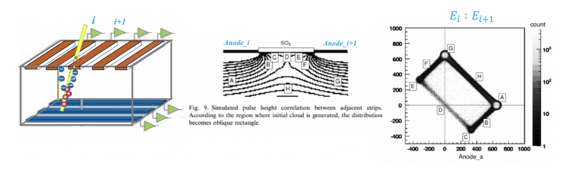
When a particle enters the interstrip region between two neighboring strips, the generated charge can be collected by both strips. A large local energy deposition may also induce a correlated signal on the adjacent strip.

The signal sharing depends on the impact position and the collection conditions inside the detector, as illustrated in the figure below (for the same deposited energy).

• The correlation between adjacent strips becomes especially complicated when low-energy incident particles, such as those from an alpha source, are stopped in the shallow region (BCDEF). For example, at positions B and F, the pulse signals induced on the two sides have opposite polarities, one positive and one negative.

• When a high-energy incident particle passes through the DSSD, as in regions A, H, and G, the signals on both sides are positive.

In routine ADC readout, positive pulses are usually recorded, so the most useful class of events is the two-strip positive-sharing event, for which the total deposited energy is approximately

$$ E = E_i + E_{i+1}. $$

These events should be reconstructed as valid cluster events rather than discarded.

Data

In the S4 data set, the Ring side has narrow strips and small spacing, so adjacent-strip correlations are more obvious there. On the pie side, the effect is much weaker. For this reason, the analysis below focuses on the Ring strips.

//%jsroot on
TFile *fin = new TFile("s4hit.root");
TTree *tree = (TTree*)fin->Get("tree");
TCanvas *c1 = new TCanvas("c1","c1",800,400);
c1->SetLogz();

Adjacent-Strip Correlation

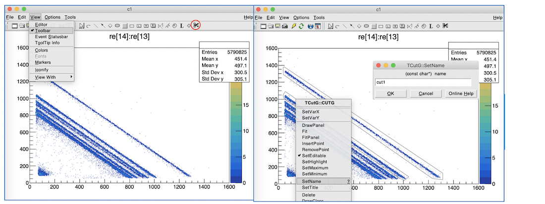
As an example, consider strips 13 and 14.

• On the Ring side, the two-dimensional plot shows a clear band with negative slope. This band corresponds to one particle sharing its energy between two adjacent strips. The pie side does not show such a strong structure.

tree->Draw("re[14]:re[13]>>hr43(800,-100,1700,800,-100,1700)","","goff");//goff 选项：只填充hist，而不显示。
tree->Draw("pe[14]:pe[13]>>hp43(800,-100,1700,800,-100,1700)","","goff");
c1->Divide(2,1);
c1->cd(1);      
hr43->Draw("colz");
c1->cd(2);       
hp43->Draw("colz");
c1->Draw();

Effect on Single-Strip Spectra

Adjacent-strip sharing broadens the spectrum of a single strip. Therefore, single-strip calibration and adjacent-strip reconstruction should be treated separately.

• The red spectrum contains events affected by adjacent-strip sharing, while the black spectrum contains isolated single-strip events. The difference between them shows why inter-strip events must be handled explicitly.

c1->Divide(1,1);
c1->cd();
tree->Draw("re[13]>>h1a(800,0,1600)","re[14]>0 || re[12]>0");// 有相邻条能量共享
TH1F *h1a = (TH1F*)gROOT->FindObject("h1a");
tree->Draw("re[13]>>h2a(800,0,1600)","re[14]<0 && re[12]<0");// 没有相邻条能量共享
h1a->SetLineColor(kRed);
h1a->Draw("same");
c1->Draw();

Selection of Two Reference Bands

Here the graphical cuts are assumed to be already prepared. Their construction is not discussed in this lecture. We only use them as event selections.

• cut1 corresponds to the $8.6931$ MeV $\alpha$ line.
• cut2 corresponds to the $6.6708$ MeV $\alpha$ line.

gROOT->Macro("cut1.C");
gROOT->Macro("cut2.C");

c1->Clear();
c1->Divide(2,1);
c1->cd(1);      
tree->Draw("re[14]:re[13]>>hcut1(800,0,1600,800,0,1600)","cut1","colz");
c1->cd(2);
tree->Draw("re[14]:re[13]>>hcut2(800,0,1600,800,0,1600)","cut2","colz");
c1->Draw();

Energy-Sharing Model

Let the ADC amplitudes of strips $i$ and $i+1$ be $A_i$ and $A_{i+1}$. Their calibrated energies are

$$ E_i = k_i A_i + b_i, \qquad E_{i+1} = k_i A_i + b_i. $$

For one particle,

$$ E = E_i + E_{i+1} = k_i A_i + k_{i+1} A_{i+1} + (b_i+b_{i+1}). $$ Therefore, the adjacent-strip correlation follows a straight line:

$$ A_{i+1} = K \cdot A_i + B, $$

with

$$ K=-\frac{k_i}{k_{i+1}}, \qquad B=\frac{E-(b_i+b_{i+1})}{k_{i+1}}. $$

Using two mono-energetic bands, we obtain $K$, $B$, and then solve for $k_i$, $k_{i+1}$, and $b_i+b_{i+1}$.

Linear Fits

• Convert TH2 to TGraph https://root.cern.ch/root/roottalk/roottalk03/0638.html

tree::Draw("x1:x2",selection);
TGraph *gr = new TGraph(tree->GetSelectedRows(), tree->GetV2(), tree->GetV1());

TGraph *gr1, *gr2;
TF1 *f1, *f2;

c1->Clear();
c1->Divide(2,1);
c1->cd(1); 

tree->Draw("re[14]:re[13]","cut1","");
gr1 = new TGraph(tree->GetSelectedRows(), tree->GetV2(), tree->GetV1());
gr1->Fit("pol1","Q");
f1 = gr1->GetFunction("pol1");
f1->Draw("same");

c1->cd(2);
tree->Draw("re[14]:re[13]","cut2","");
gr2 = new TGraph(tree->GetSelectedRows(), tree->GetV2(), tree->GetV1());
gr2->Fit("pol1","Q");
f2 = gr2->GetFunction("pol1");
f2->Draw("same");
c1->Draw();

Parameter Extraction

double E1 = 8.6931;
double E2 = 6.6708;
double K13,K14,K,B13,B14,k13,k14,b13_14;

K13 = f1->GetParameter(1);
K14 = f2->GetParameter(1);
K  = (K13 + K14)/2.0;

B13 = f1->GetParameter(0);
B14 = f2->GetParameter(0);

k14  = (E1-E2)/(B13-B14);
k13  = -K*k14;
b13_14 = E1 - k14*B13;

cout << Form("k13 = %f, k14 = %f, b13 + b14 = %f",k13,k14,b13_14) << endl;

k13 = 0.007014, k14 = 0.006918, b13 + b14 = -0.826077

Energy Reconstruction

After reconstruction, the shared events are converted into a total-energy spectrum. In practical analysis, this is the key step: identify the adjacent-strip event, reconstruct the cluster energy, and then keep the event in the later analysis chain. Recent detector studies also show that interstrip events can be reconstructed effectively rather than treated as unusable events.

tree->SetAlias("e13_14",Form("%f*re[13] + %f*re[14] - %f",k13,k14,b13_14));
tree->Draw("e13_14>>hsum(2000,0,10)","re[13]>0 && re[14]>0");
c1->Draw();

Position Reconstruction

An adjacent-strip event should not be treated automatically as a particle hitting exactly at the geometrical gap. In real data, two neighboring strips may fire because of true interstrip charge sharing, but also because of impact position, impact angle, coupling, or other detector-response effects. The useful subset is the clean two-strip sharing event.

For position analysis, the practical rule is simple:

• exactly two adjacent strips carry the signal;
• both signals are positive and above threshold;
• no extra neighboring strip participates;
• the summed energy is consistent with one particle.

For such events, the charge ratio contains position information inside one strip pitch. A simple position estimator is the energy-weighted centroid,

$$ x_c=\frac{E_i x_i + E_{i+1} x_{i+1}}{E_i+E_{i+1}}. $$

This gives a continuous position estimate and is more informative than assigning the event only to the strip with the larger signal. In this sense, clean adjacent-strip events can be used for position refinement beyond the digital strip index, while still preserving the deposited energy.