3.1 DSSD Energy Calibration
DSSD 探测器
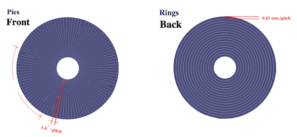
Detectors: S4
128(Pie) x 128(Ring)
Pie: $1.4^{\circ}$/条, HV=-110V
Ring: 0.43 mm 条宽,~0.03 mm 条间距, HV=0V
厚度1014 $\mu$m
放射源
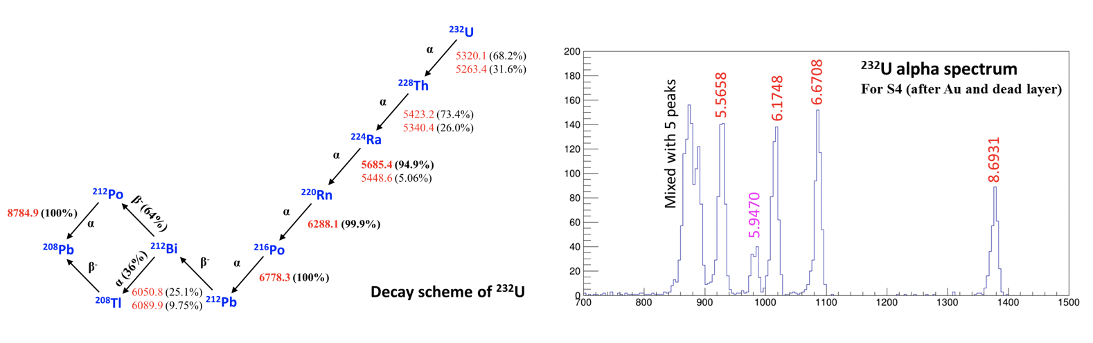
$\alpha-$Sources: $^{232}U$
$\alpha$粒子从Pie面入射,考虑放射源表面的金膜和Si前表面的死层后,最终沉积在Si里的能量分别为 $5.5658$ MeV, $6.1748$ MeV, $6.6708$ MeV, $8.6931$ MeV.
使用下图中标红色的4个峰进行刻度.
- 数据: s4.root
- 数据是用Digital modules的自触发模式记录的, 数据截取了pie和ring的前48条信息。
 Int_t pe[48];//Pie 0-48
 Int_t re[48];//Ring 0-48
TFile *f = new TFile("s4.root");
TTree *tree = (TTree*)f->Get("tree");
TCanvas *c1 = new TCanvas;
tree->Draw("pe[0]>>hx0(1000, 0, 2000)");//单条
tree->Draw("pe[1]>>hx1(1000, 0, 2000)");//单条
TH1I *hx0 = (TH1I*)gROOT->FindObject("hx0");
TH1I *hx1 = (TH1I*)gROOT->FindObject("hx1");
hx0->SetLineColor(kGreen);
hx1->Draw();
hx0->Draw("same");
c1->Draw();
tree->Draw("pe>>(1000,0,2000)");//所有条pe[0-48]累积
c1->Draw();
tree->Draw("re[0]>>hy0(1000, 0, 2000)");//单条
tree->Draw("re[1]>>hy1(1000, 0, 2000)");//单条
TH1I *hy0 = (TH1I*)gROOT->FindObject("hy0");
TH1I *hy1 = (TH1I*)gROOT->FindObject("hy1");
gPad->SetLogy();
hy0->SetLineColor(kGreen);
hy1->Draw();
hy0->Draw("same");
c1->Draw();
TSpectrum
TSpectrum 用于一维谱分析中的几个核心问题:本底估计、平滑、反卷积和寻峰。在刻度问题中,最直接相关的是本底估计和寻峰。(zhihuanli.github.io)
创建对象时需要先给出允许搜索的最大峰数,例如: 创建对象时需要先给出允许搜索的最大峰数,例如:
TSpectrum *s = new TSpectrum(500);
这个数字不是实际峰数,而是允许搜索的上限。(zhihuanli.github.io)
Background
用于本底估计的接口可以写成:
TH1 *TSpectrum::Background(const TH1 *h,
                           Int_t niter = 20,
                           Option_t *option = "");
其中 niter 控制本底的平滑程度。一般来说,niter 越大,本底越平滑,也越容易压低;但本底减除不能过度,否则会侵入真实峰区,甚至在峰区附近产生不合理的负值。这里的原则是让本底足够平滑,同时尽量不破坏真实峰形。
先由 Background 构造本底,再从原谱中减去本底,得到更适合后续寻峰的谱。
TFile *f = new TFile("gamma.root");
TH1F *h0 = (TH1F*)f->Get("h0");

TSpectrum *s = new TSpectrum(500);
TH1F *hbg = (TH1F*)s->Background(h0, 30, "same");
TH1F *hpeak  = (TH1F*)h0->Clone("hh");
hpeak->Add(hpeak, hbg, 1, -1);
hpeak->SetName("hpeak");
c1->Clear();
h0->SetLineColor(kBlack);
hbg->SetLineColor(kRed);
hpeak->SetLineColor(kBlue);
hpeak->Draw();
h0->Draw("same");
hbg->Draw("same");
gPad->SetLogy();
c1->Draw();
Search
用于自动找峰的接口可以写成:
Int_t TSpectrum::Search(const TH1 *hin,
                        Double_t sigma = 2,
                        Option_t *option = "",
                        Double_t threshold = 0.05);
其中 sigma 反映待寻找峰的大致宽度,threshold 是一个相对阈值,用于丢弃低于最高峰一定比例的小峰。减小 threshold 会明显增加候选峰数,因此它控制的不是“真峰还是假峰”的绝对分界,而是“候选峰集”的大小。
Double_t *xpeaks = nullptr;
Double_t *ypeaks = nullptr;

Int_t nfound = s->Search(hpeak, 2, "", 0.01);

xpeaks = s->GetPositionX();
ypeaks = s->GetPositionY();

cout << nfound << endl;
for(int i=0; i<nfound; i++)
    cout << i << ": " << int(xpeaks[i])
         << ", " << ypeaks[i] << endl;
hpeak->Draw();
c1->Draw();
18
0: 332, 984052
1: 135, 786091
2: 101, 664539
3: 322, 538447
4: 67, 355974
5: 288, 331300
6: 239, 171454
7: 688, 161288
8: 1217, 167250
9: 843, 152510
10: 356, 139327
11: 265, 136479
12: 968, 127081
13: 71, 117777
14: 946, 100460
15: 406, 53913
16: 762, 46709.3
17: 379, 38620.6
std::vector
自动找峰之后,候选峰的个数并不固定,因此不适合用固定长度数组存放。这里使用 std::vector,把每一条谱上找到的候选峰位收集起来。它和数组一样可以按下标访问,但长度可变,更适合寻峰结果。
常用写法如下:
#include <vector>
#include <algorithm>
using namespace std;

vector<Double_t> pe;
pe.push_back(993);
pe.push_back(1079);

for (int i=0; i<pe.size(); i++) {
    cout << i << " " << pe[i] << endl;
}

for (auto it = pe.begin(); it != pe.end(); ++it) {
    cout << *it << endl;
}
在这一节,vector<Double_t> 用来保存某一条 Pie 谱上全部候选峰的位置,供后续匹配和拟合使用。
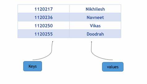
std::map 与 std::multimap
找到候选峰之后,下一步不是按返回顺序直接使用,而是要按某个更有物理意义的量重新组织。这里用到 map 和 multimap。它们都会按 key 自动排序,其中 map 的 key 不能重复,而 multimap 允许多个相同 key。
- 在
map或multimap中插入元素可用insert(make_pair(key, value)),也可用emplace(key, value);后者直接在容器内构造元素,写法更简洁,在解释环境中也通常更稳。
基本形式可以写成:
#include <map>
using namespace std;

map<Int_t, Double_t> m1;
multimap<Int_t, Double_t> mm1;

// 插入元素可用 insert(make_pair(key, value))
m1.insert(make_pair(762, 121.78));

// 也可用 emplace(key, value)
mm1.emplace(1560, 1079.0);
mm1.emplace(1550,  993.0);
mm1.emplace(1494, 1147.0);

//常见操作包括 `insert`、`find`、正向遍历和反向遍历:

```cpp
auto im1 = m1.find(762);
if(im1 != m1.end()) {
    cout << im1->first << " " << im1->second << endl;
}

for(auto it = mm1.begin(); it != mm1.end(); ++it) {
    cout << it->first << " " << it->second << endl;
}

for(auto it = mm1.rbegin(); it != mm1.rend(); ++it) {
    cout << it->first << " " << it->second << endl;
}
在刻度问题中,最自然的做法是把峰高作为 key、峰位作为 value,写成 multimap<Int_t, Double_t>。这样即使多个峰高度接近甚至相同,也都能保留下来;再通过反向遍历,就能按峰高从大到小提取候选峰。
寻峰函数 peaks.C
为了把自动找峰写成一个可复用步骤,可以把它整理成一个函数。输入是直方图名字,输出是一个 vector<Double_t>;其中峰位按峰高从大到小保存。函数内部用 TSpectrum::Search 寻峰,用 multimap 完成“峰高—峰位”的重排,并把峰位标到图上。
TH1F *h = NULL, *hb = NULL;

void peaks(TString hname, vector<Double_t> &pe, Double_t thres=0.05, int backsub=1)
{
  Int_t nfound;
  Double_t *xpeaks = NULL, *ypeaks = NULL;
  pe.clear();

  multimap<Double_t, Double_t> me;   // key: ypeaks, value: xpeaks

  h = (TH1F*)gROOT->FindObject(hname);
  if(!h) {
    cout << "Histogram " << hname << " not found." << endl;
    return;
  }

  TSpectrum *sp = new TSpectrum(500);

  if(backsub) {
    hb = (TH1F*)sp->Background(h, 80);
    h->Add(h, hb, 1, -1);
  }

  nfound = sp->Search(h, 2, "", thres);

  TPolyMarker *pm = (TPolyMarker*)h->GetListOfFunctions()->FindObject("TPolyMarker");
  if(pm) {
    pm->SetMarkerStyle(32);
    pm->SetMarkerColor(kGreen);
    pm->SetMarkerSize(0.4);
  }

  xpeaks = sp->GetPositionX();
  ypeaks = sp->GetPositionY();

  for(int j=0; j<nfound; j++) {
    me.emplace(ypeaks[j], xpeaks[j]);

    TLatex *tex = new TLatex(xpeaks[j], ypeaks[j], Form("%.0f", xpeaks[j]));
    tex->SetTextFont(13);
    tex->SetTextSize(0.02);
    tex->SetTextAlign(12);
    tex->SetTextAngle(90);
    tex->SetTextColor(kRed);
    tex->Draw();
  }

  for(auto ie = me.rbegin(); ie != me.rend(); ++ie) {
    cout << ie->second << " " << ie->first << endl;
    pe.push_back(ie->second);
  }

  delete sp;
}
这一步非常关键。TSpectrum 负责“找到所有可能峰”,vector 负责“保存个数不固定的结果”,multimap 负责“按峰高重新组织候选峰”。三者在这里第一次组成一个完整的分析单元。
cout<<hpeak->GetName()<<endl;
hpeak
gROOT->ProcessLine(".L peaks.C");
vector<Double_t> ge;
peaks("hpeak",ge);
gPad->SetLogy(0);
c1->Draw();
332.7 984184
135.9 786218
101.7 664645
322.9 538568
67.1 356220
288.1 331398
239.1 171570
1217.1 167254
688.3 161309
843.9 152524
356.1 139455
265.9 136580
968.3 127103
71.9 117995
946.3 100477
406.7 53964
DSSD Energy Calibration
对某一条 Pie 谱执行:
TFile *f = new TFile("s4.root");
TTree *tree = (TTree*)f->Get("tree");
tree->Draw("pe[1]>>hx1(1000, 0, 2000)");//单条
gROOT->ProcessLine(".L peaks.C");//可以在代码内部直接使用,等价于[ROOT >] .L peaks.C
vector<Double_t> pe;
Double_t e[4] = {5.5658, 6.1748, 6.6708, 8.6931};//alpha energy
Info in <TCanvas::MakeDefCanvas>: created default TCanvas with name c1
peaks("hx1", pe);
gPad->SetLogy(0);
c1->Draw();
941 1750.78
1079 1558.87
993 1549.81
1147 1493.93
957 1358.79
1429 604.009
1047 479.849
277 238.949
1405 133.009
此时得到的是一组候选峰位。对示例谱而言,较显著的峰位包括 941、957、993、1079、1147、1429 等。这里真正的问题不是“有没有找到峰”,而是“哪 4 个峰与已知的 4 个 $\alpha$ 能量对应”。
在这条谱中,993、1079、1147、1429 是最可能与已知$\alpha$ 能量匹配的一组,但仅凭峰高并不能完全确定顺序。原因有两点:一是这些峰的高度相差不大;二是当分辨较差时,941 和 957 还可能并成一个峰。因此,不能把寻峰结果直接等同于最终刻度峰。
候选峰与已知能量的匹配
对当前谱,可以先采用一个针对谱形的经验策略:取前 6 个显著峰,按峰位排序,再取其中 4 个与已知能量做匹配。 这样得到的峰位是 993、1079、1147、1429。对应的思路是:先利用寻峰和峰高排序缩小候选范围,再结合谱形和已知刻度点选出最合理的一组。
更一般的策略是:把 TSpectrum 给出的候选峰与 4 个已知 $\alpha$ 能量进行组合,分别做线性拟合,比较每一组的 $\chi^2/\mathrm{NDF}$,取最小的一组作为实际的峰位—能量组合。这种策略不依赖某一条谱的具体形状,更适合推广到全部 48 条。
sort(pe.begin(),pe.begin()+6);
Double_t mpe[4], cpe[4];//peak,count
for(int i=0; i<4; i++) {
    mpe[i] = pe[2+i];
    cpe[i] = hx1->GetBinContent(hx1->FindBin(mpe[i]));
    cout << mpe[i] << " " << cpe[i] << endl;
}
993 1549.81
1079 1558.87
1147 1493.93
1429 604.009
粗刻度
选定 4 个候选峰位以后,可以先做一轮峰位—能量线性拟合,得到粗刻度关系:
TGraph *gr = new TGraph(4, mpe, e);
gr->Draw("A*");
gr->Fit("pol1");
TF1 *f1 = gr->GetFunction("pol1");
c1->Draw();
****************************************
Minimizer is Linear / Migrad
Chi2                      =  4.40562e-05
NDf                       =            2
p0                        =     -1.56557   +/-   0.0168397
p1                        =   0.00717874   +/-   1.43506e-05
Double_t p0 = f1->GetParameter(0);
Double_t p1 = f1->GetParameter(1);
Double_t dpe[4];
for(int i=0; i<4; i++)
    dpe[i] = p0 + p1 * mpe[i] - e[i];
TGraph *rgr = new TGraph(4,mpe,dpe);
rgr->Draw("A*");
c1->Draw();
hx1->Draw();
c1->Draw();
double par[4][3];//peak,sigma,chi2/ndf
double ge[4];
TF1 *fg[4];
TFitResultPtr fr;
for(int i=0; i<4; i++) {
    fg[i] = new TF1(Form("fg%d", i), "gaus");
    fg[i]->SetParameters(cpe[i], mpe[i], 4);//constant,mean, sigma
    fr = hx1->Fit(fg[i], "SQ+", "", mpe[i]-5, mpe[i]+8);//superimpose TF1 to hx1
    par[i][0] = fg[i]->GetParameter(1);
    par[i][1] = fg[i]->GetParameter(2);
    par[i][2] = fr->Chi2()/fr->Ndf();
    ge[i] = par[i][0];
    cout << Form("peaks = %4.1f, sigma = %.2f, chi2/ndf = %.2f",
                 par[i][0], par[i][1], par[i][2]) << endl;
}
c1->Draw();
peaks = 992.9, sigma = 3.98, chi2/ndf = 12.92
peaks = 1078.3, sigma = 4.00, chi2/ndf = 11.31
peaks = 1147.3, sigma = 3.98, chi2/ndf = 13.36
peaks = 1429.0, sigma = 4.83, chi2/ndf = 1.27
TGraph *gr1 = new TGraph(4,ge,e);
gr1->Draw("A*");
gr1->Fit("pol1");
TF1 *f2 = gr->GetFunction("pol1");
c1->Draw();
****************************************
Minimizer is Linear / Migrad
Chi2                      =  5.94481e-06
NDf                       =            2
p0                        =     -1.55862   +/-   0.00618078
p1                        =   0.00717354   +/-   5.26767e-06
p0 = f2->GetParameter(0);
p1 = f1->GetParameter(1);
for(int i=0; i<4; i++)
    dpe[i] = p0 + p1 * ge[i] - e[i];
TGraph *rgr1 = new TGraph(4, ge, dpe);
rgr1->Draw("A*");
c1->Draw();
tree->Draw(Form("pe[0]*%f+%f>>hx1e(1000, -1, 10)", p1, p0));//单条
hx1e->Draw();
c1->Draw();//存在锯齿,需要在刻度前进行连续化。