2.1 PPAC 信号处理-I

1. PPAC

• 电离与雪崩：带电粒子穿过 PPAC 的工作气体（通常为 $C_3F_8$ 或 $C_4H_{10}$），在路径上产生初级电离。电子在强电场作用下向阳极漂移并发生 Townsend 雪崩。
• 感应信号：
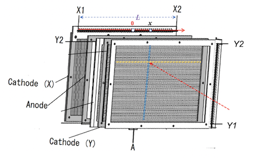
  • 阳极 (Anode)：一整块薄镀铝 Mylar 膜。雪崩电子被阳极收集，产生快速的时间信号 $t_a$，作为该粒子到达 PPAC 的参考时间。
  • 阴极 (Cathode)：分成 1mm 间隔的读数条 (Strips)，X 和 Y 方向正交。阳极上的雪崩会在阴极条上产生感应电荷信号。

Delay-line 读出原理

阴极条之间通过高精度的电磁延迟线（Delay Line）连接。感应信号会沿延迟线向两端传输。

• $T_{xdelay}/T_{ydelay}$：信号在x/y方向延迟线上的总传播时间（常数）。
• $Q$：感应信号的幅度。

假设粒子击中位置为 $x$ (以中心为0)，延迟线总长度为 $L$，信号在延迟线内部传输时间（设信号传输速度 $v_d = L/T_{xdelay}$）： $$ \begin{align} &T_{xdelay} = t_{x1} + t_{x2} \\ &t_{x1} = \left(\frac{L}{2} + x \right) \frac{T_{xdelay}}{L} \\ &t_{x2} = \left(\frac{L}{2} - x \right) \frac{T_{xdelay}}{L} \\ &x = (t_{x2} - t_{x1}) \frac{L}{2 T_{xdelay}} \end{align} $$

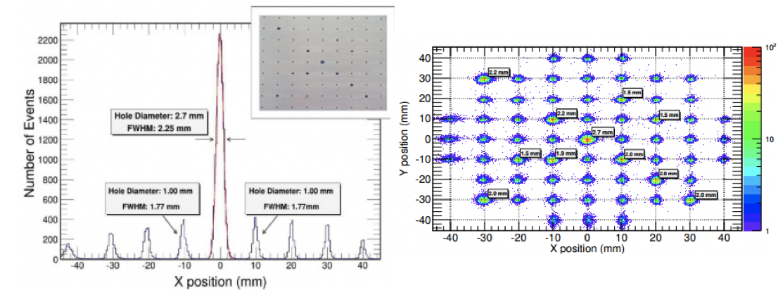
PPAC Position Calibration

• 将 $\alpha$-放射源置于远处，$\alpha$ 粒子入射到盖有 Mask 的探测器上（Mask上孔的位置分布已知），得到 x 方向和 y 方向的一系列峰位。通过拟合时间差谱 $(\Delta t_{x2} - \Delta t_{x1})$ 的峰位和实际物理位置，得到刻度系数 $k = L / 2T_{xdelay}$。
• 探测器安装到束流线后，通过位置测量，确定探测器中心相对于束流中心线的偏移 $b$。
• 实验中，通过测量经过中心线的束流（利用限制束流线上的 slit 狭缝），进一步检验和校准上述偏移。

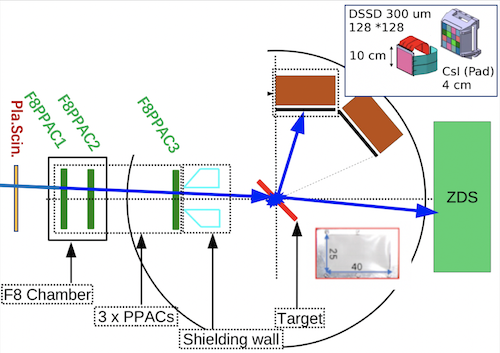
2. 实验设置:

实验中，F8PPAC1-3 用于测量靶前束流的入射方向和轨迹。靶后有两套探测系统：

1. MUST2 望远镜系统：测量反应产生的轻粒子。
2. 零度磁谱仪 (ZDS)：探测剩余重核。

几何布局优化： 为了减少散射粒子在靶内的能量损失，靶框被旋转 45° 朝向望远镜摆放。靶前放置了由厚铁块组成的屏蔽体，用于阻挡束流晕（Beam Halo），避免偏离中心线的非物理粒子击中靶后的探测系统。

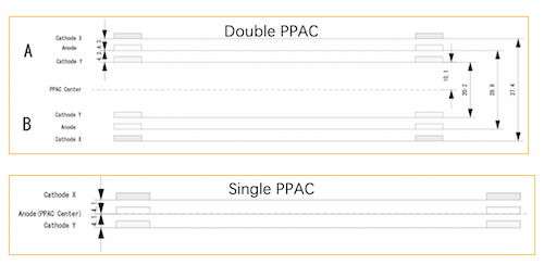
两种类型 PPAC

实验中采用了两种不同规格尺寸的 PPAC：

• 一种是 double PPAC (F8PPAC1, F8PPAC2)，面积为 $240 \times 150 \text{ mm}^2$。
• 另一种是 single PPAC (F8PPAC3)，面积为 $100 \times 100 \text{ mm}^2$。

实际PPAC 信号

• Trigger (time start): Plastic scintillator (塑闪)
• 飞行时间 ($TOF$)：粒子从塑闪飞到 PPAC 的时间
• 阴极，阳极信号的 offset：$t_{off,x1}，t_{off,x2}，t_{off,a}$
• TDC 记录的绝对时间信号：$T_{x1}，T_{x2}，T_a$

阴极时间 (包含束流速度依赖性)

TDC 记录的时间不仅包含了信号在探测器内的传输时间，还包含了粒子的飞行时间 ($TOF$) 和硬件 offset：

• $T_{x1} = TOF + t_{x1} + t_{off,x1}$
• $T_{x2} = TOF + t_{x2} + t_{off,x2}$
• $T_{x1} + T_{x2} = 2 TOF + T_{xdelay} + (t_{off,x1} + t_{off,x2})$
• $T_{x1} - T_{x2} = t_{x1} - t_{x2} + (t_{off,x1} - t_{off,x2})$

阳极时间

• $T_a = TOF + t_{off,a}$

组合参数 (相对时间，消除速度依赖性)

上述绝对时间信号不仅与探测器内部传输有关，也与束流的到达时间 ($TOF$) 有关。研究探测器特征时，必须消除束流动量弥散带来的 $TOF$ 展宽。 通过将阴极信号减去阳极信号，可以抵消 $TOF$的影响：

• $\Delta T_{x1} = T_{x1} - T_a = t_{x1} + (t_{off,x1} - t_{off,a})$
• $\Delta T_{x2} = T_{x2} - T_a = t_{x2} + (t_{off,x2} - t_{off,a})$
• $\Delta T_{x1} - \Delta T_{x2} = t_{x1} - t_{x2} + (t_{off,x1} - t_{off,x2})$

探测器两端信号关联

• $\mathbf{T_{x1} + T_{x2}} = 2 TOF + Const.$ (包含 $TOF$，与束流速度有关，分布表现为一个较宽的峰)
• $\mathbf{\Delta T_{x1} + \Delta T_{x2}} = t_{x1} + t_{x2} + (t_{off,x1} + t_{off,x2} - 2t_{off,a}) = T_{xelay} + Const. = \mathbf{Const.}$ (与束流速度无关，分布表现为一个极窄的峰，直接反映探测器本征时间分辨率)

文件中 TreeBranch 的定义

• Trigger = beamTrig + must2Trig
  • beamTrig=1，由靶前塑闪探测器触发（束流的取样触发）。
  • must2Trig=1，由靶后 MUST2 望远镜信号触发（即物理事件符合触发）。
• F8PPACRawData[i][j] - Raw Data (原始信息，TDC 道值)

Branch	PPAC
F8PPACRawData[0][0]	PPAC 1 Layer A $T_{x1}$
F8PPACRawData[0][1]	PPAC 1 Layer A $T_{x2}$
F8PPACRawData[0][2]	PPAC 1 Layer A $T_{y1}$
F8PPACRawData[0][3]	PPAC 1 Layer A $T_{y2}$
F8PPACRawData[0][4]	PPAC 1 Layer A $T_a$
F8PPACRawData[1][0-4]	PPAC 1 Layer B
F8PPACRawData[2][0-4]	PPAC 2 Layer A
F8PPACRawData[3][0-4]	PPAC 2 Layer B
F8PPACRawData[4][0-4]	PPAC 3

数据分析

观察原始变量，确定合理范围

• 合理信号范围：0 < t < 4095

//%jsroot on
TFile *ipf = new TFile("f8ppac001.root");//  $HOME/data/MUST2@BigRIPS/ROOTFILE/
TTree *tree = (TTree*) ipf->Get("tree");
TCanvas *c1 = new TCanvas;

t_x1/t_x2

tree->Draw("F8PPACRawData[0][0] >> h_raw_tx1(1000, 0, 4200)");
tree->Draw("F8PPACRawData[0][1] >> h_raw_tx2(1000, 0, 4200)","","same");
c1->SetLogy();
c1->Draw();

t_y1/t_y2

tree->Draw("F8PPACRawData[0][2] >> h_raw_ty1(1000, 0, 4200)");
tree->Draw("F8PPACRawData[0][3] >> h_raw_ty2(1000, 0, 4200)","","same");
c1->SetLogy();
c1->Draw();

ta

tree->Draw("F8PPACRawData[0][4]>>hraw_ta(1000,0,4200)");//F8PPAC1A-Ta
c1->Draw();

组合参数

• SetAlias : 设置别名

tree->SetAlias("t_x1", "F8PPACRawData[0][0]");
tree->SetAlias("t_x2", "F8PPACRawData[0][1]");
tree->SetAlias("t_y1", "F8PPACRawData[0][2]");
tree->SetAlias("t_y2", "F8PPACRawData[0][3]");

tree->SetAlias("t_a",  "F8PPACRawData[0][4]");
tree->SetAlias("dt_x1", "(t_x1 - t_a)");
tree->SetAlias("dt_x2", "(t_x2 - t_a)");
tree->SetAlias("dt_y1", "(t_y1 - t_a)");
tree->SetAlias("dt_y2", "(t_y2 - t_a)");

TCut cut_xvalid = "t_a>10 && t_a<4000 && t_x1>10 && t_x1<4000 && t_x2>10 && t_x2<4000";
TCut cut_yvalid = "t_a>10 && t_a<4000 && t_y1>10 && t_y1<4000 && t_y2>10 && t_y2<4000";

dt_x1/dt_x2

tree->Draw("dt_x1 >> h1_dtx1(2000, -4000, 4000)", cut_xvalid);
tree->Draw("dt_x2 >> h1_dtx2(2000, -4000, 4000)", cut_xvalid, "same");
c1->SetLogy();
c1->Draw();

dt_x2 : dt_x1

• $\mathbf{\Delta T_{x1} + \Delta T_{x2}} = T_{xdelay} + Const. = \mathbf{Const.}$

dt_y2 : dt_y1

• $\mathbf{\Delta T_{y1} + \Delta T_{y2}} = T_{ydelay} + Const. = \mathbf{Const.}$

TCanvas *c3 = new TCanvas("c3","c3",1000,400);
c3->Divide(2,1);
c3->cd(1);
tree->Draw("dt_x2 : dt_x1 >> h2_corrx(1000, -2000, 2000, 1000, -2000, 2000)", cut_xvalid, "colz");
TLine *tlx1 = new TLine(-200,1410,1420,-200);
TLine *tlx2 = new TLine(-200,1330,1340,-200);
tlx1->SetLineColor(kRed);
tlx2->SetLineColor(kRed);
tlx1->Draw("same");
tlx2->Draw("same");

c3->cd(2);
tree->Draw("dt_y2 : dt_y1 >> h2_corry(1000, -2000, 2000, 1000, -2000, 2000)", cut_yvalid, "colz");
TLine *tly1 = new TLine(-200,900,900,-200);
TLine *tly2 = new TLine(-200,820,820,-200);
tly1->SetLineColor(kRed);
tly2->SetLineColor(kRed);
tly1->Draw("same");
tly2->Draw("same");

c3->SetLogy(0);
c3->Draw();

TCanvas *c4 = new TCanvas("c4","c4",1000,400);
c4->Divide(2,1);
c4->cd(1);
tree->Draw("dt_x2 + dt_x1 >> hdt_xsum(1500, 0, 1500)", cut_xvalid, "colz");
TH1D *hdt_xsum = (TH1D*)gROOT->FindObject("hdt_xsum");
hdt_xsum->Fit("gaus","Q");
TF1 *fx = hdt_xsum->GetFunction("gaus");
Float_t xpeak = fx->GetParameter(1);
Float_t xsigma = fx->GetParameter(2);
cout << "xpeak = " << xpeak << " xsigma = "<<xsigma << endl;
gPad->SetLogy();

c4->cd(2);
tree->Draw("dt_y2 + dt_y1 >> hdt_ysum(1500, 0, 1500)", cut_yvalid, "colz");
TH1D *hdt_ysum = (TH1D*)gROOT->FindObject("hdt_ysum");
hdt_ysum->Fit("gaus","Q");
TF1 *fy = hdt_ysum->GetFunction("gaus");
Float_t ypeak = fy->GetParameter(1);
Float_t ysigma = fy->GetParameter(2);
cout << "ypeak = " << ypeak << " ysigma = "<<ysigma << endl;
gPad->SetLogy();
c4->Draw();

xpeak = 1172.2 xsigma = 7.98306
ypeak = 662.065 ysigma = 9.00337

Pileup Cut

• 当同时有2个或以上的粒子打在 PPAC 上时，到达 delayline 的 x 的两端的时间由不同粒子的信号给出。

  • 假设 a, b 粒子同时穿过探测器，且 a 粒子靠近 $x_1$ 侧，b 粒子靠近 $x_2$ 侧，则 $T_{x_1}$ 由 a 粒子给出，$T_{x_2}$ 则由 b 粒子给出。 (TDC 只记录与 start 信号最近的第一个信号)。

• 此时，$T_{x_1}+T_{x_2} < T_{delay}$。即 delayline 的两端信号传输时间之和不再是常数。这个条件可作为信号堆积的标志。

• 从上述讨论可知，PPAC 无堆积条件：前后两个粒子到达探测器的时间间隔大于 $T_{delay}$。

• 一般选择加合峰（正常单粒子事件）两侧三倍 $\sigma$ 的范围作为好事件的筛选条件，剔除范围外的堆积信号：`

TString scut_xpile = Form("abs(dt_x2 + dt_x1 - %f) < 3 * %f", xpeak, xsigma);
TString scut_ypile = Form("abs(dt_y2 + dt_y1 - %f) < 3 * %f", ypeak, ysigma);

TCut cut_xpile = scut_xpile.Data() && cut_xvalid; 
TCut cut_ypile = scut_ypile.Data() && cut_yvalid; 
TCut cut_xypile = cut_xpile && cut_ypile;

TCanvas *c1 = new TCanvas;
tree->Draw("dt_y1-dt_y2:dt_x1-dt_x2",cut_xypile, "colz");
gPad->SetLogy(0);
gPad->SetLogz();
c1->Draw();