ROOT III Example — Telescope
This example connects several ROOT techniques to a simple nuclear-physics application: energy loss of carbon ions in silicon detectors and the response of a silicon telescope.
Before doing the ROOT calculation, we first summarize the necessary physics background: stopping power, its main parameter dependence, and the principle of the $\Delta E-E$ telescope.
Background: Stopping power
When a charged particle passes through matter, it loses kinetic energy mainly through ionization and excitation of atoms in the material. The average energy loss per unit path length is called the stopping power:
$$ -\frac{dE}{dx} $$
For heavy charged particles, the stopping power is approximately described by the Bethe formula:
$$ -\frac{dE}{dx} = K\,\frac{z^2}{\beta^2}\,\rho \frac{Z}{A} \left[ \frac{1}{2}\ln\!\left(\frac{2m_e c^2 \beta^2\gamma^2 T_{\max}}{I^2}\right) -\beta^2 -\frac{\delta(\beta)}{2} -\frac{C}{Z} \right] $$
where:
- $z$: charge number of the incident particle
- $Z$, $A$: atomic number and mass number of the absorber material
- $\rho$: density of the material
- $\beta = v/c$, $\gamma = 1/\sqrt{1-\beta^2}$
- $I$: mean excitation energy of the absorber
- $T_{\max}$: maximum transferable energy in a single collision
- $\delta$: density-effect correction
- $C/Z$: shell correction
- $K$: a constant
For this lecture, it is not necessary to remember the full formula. The important point is to understand the main physical dependences of $dE/dx$.
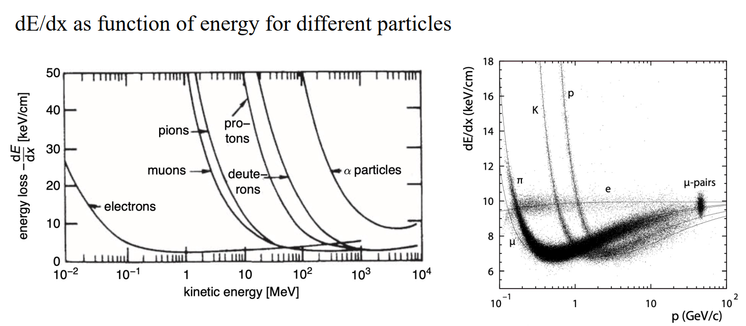
Main dependences of $dE/dx$
From the stopping-power formula, we can summarize several important features.
Dependence on particle charge
The stopping power is approximately proportional to
$$ z^2 $$
so particles with larger charge lose energy more strongly.
Dependence on particle velocity
The stopping power depends strongly on the particle speed.
At relatively low energy, a useful approximation is
$$ -\frac{dE}{dx} \propto \frac{1}{v^2} $$
so slower particles lose energy more strongly.
At higher energy, the logarithmic term changes slowly with velocity, and the energy dependence becomes weaker.
Dependence on the absorber material
The stopping power is also roughly proportional to
$$ \rho \frac{Z}{A} $$
so it depends on the density and composition of the material.
Dependence on particle mass
For fixed charge $z$ and fixed velocity $v$, the stopping power is approximately independent of the mass of the incident particle.
This point is especially useful when discussing isotopes.
Isotopes and the $E/A$ description
For non-relativistic ions,
$$ E \propto A v^2 $$
so
$$ v^2 \propto \frac{E}{A} $$
Therefore, isotopes of the same element with the same energy per nucleon $E/A$ have approximately the same velocity $v$, and hence approximately the same stopping power.
This leads to an important practical rule:
For isotopes with the same $Z$, the stopping power can be treated approximately as a function of $E/A$.
For example, if $^{4}\mathrm{He}$, $^{6}\mathrm{He}$, and $^{8}\mathrm{He}$ have the same $E/A$, then they have approximately the same $-dE/dx$.
This is why stopping-power and range tables are often given in MeV/u. In practice, one can use the same $dE/dx(E/A)$ or range curve for isotopes of the same element as a first approximation.
Practical note: why we usually use databases or simulation codes
Although the Bethe formula gives the basic physical picture, actual energy-loss calculations are usually more complicated than the simple analytic expression shown above.
In realistic calculations, one often needs to consider effects such as:
- effective charge of the ion at low energy
- shell correction and density-effect correction
- deviations from the simple Bethe form at low and intermediate energy
- energy-loss straggling
- multiple scattering
- nuclear reactions in the material
- detector dead layers and non-uniformities
In addition, practical stopping-power calculations often rely on:
- more detailed physical models
- multi-step numerical procedures
- interpolation and extrapolation based on experimental databases
For this reason, in real applications one usually reads stopping or range data from dedicated software packages or tabulated databases, rather than calculating everything directly from the basic formula. This is the approach used in this lecture.
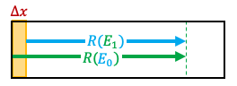
Thin-detector approximation
For a thin detector of thickness $\Delta x$, the deposited energy is approximately
$$ \Delta E \approx \left(\frac{dE}{dx}\right)\Delta x $$
If the logarithmic term changes slowly, then one may write approximately
$$ \frac{dE}{dx} \propto \frac{z^2}{v^2} $$
Using
$$ E \propto A v^2 $$
we obtain the rough relation
$$ \frac{dE}{dx} \propto \frac{A z^2}{E} $$
This relation is very useful for understanding particle identification qualitatively:
- particles with different $z$ lose different amounts of energy
- particles with different $A$ but the same total energy also behave differently
- lower-energy particles generally lose more energy in a thin detector
This is the physical basis of the $\Delta E-E$ method.
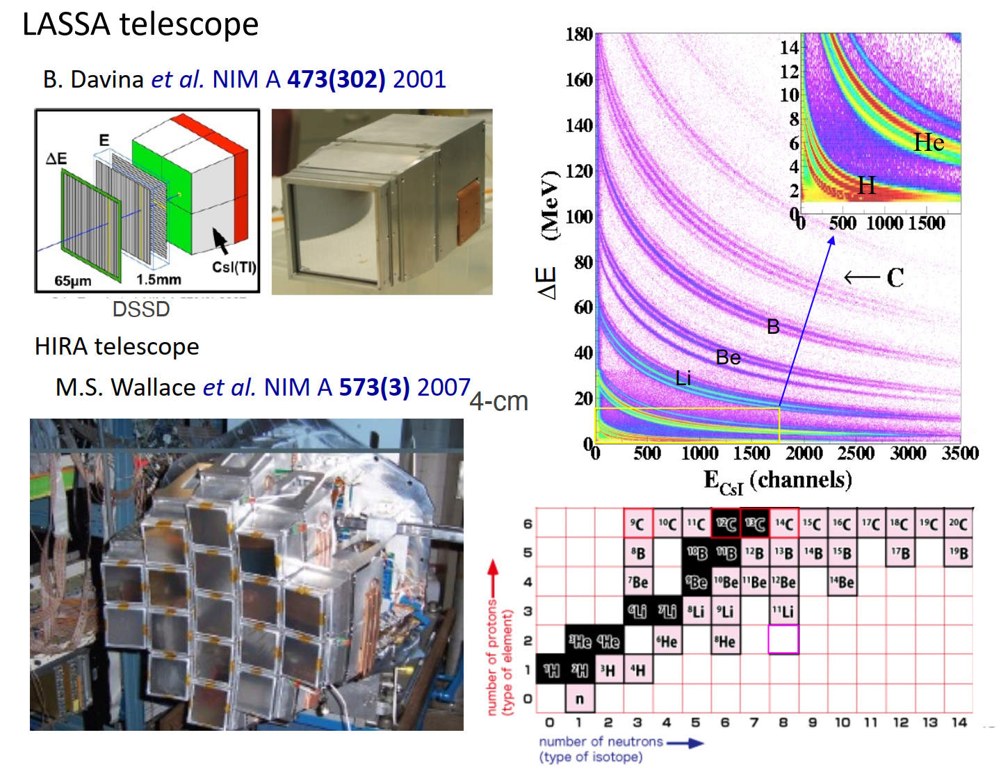
Principle of a telescope detector
A telescope detector usually consists of:
- one or more thin detectors in front, measuring $\Delta E$
- one thicker detector behind, measuring the residual energy $E$
The idea is simple:
- the front detector records how much energy the particle loses at the beginning of its path
- the back detector records how much energy remains after that loss
Because the stopping power depends on the particle charge, velocity, and mass-to-energy relation, different particles produce different correlations between $\Delta E$ and $E$.
Therefore, in a two-dimensional plot such as
$$ \Delta E \text{ vs } E $$
different particle species form different bands or loci. This is why silicon telescopes are widely used for particle identification in nuclear-physics experiments.
In an ideal case:
- the front detector is thin enough that it measures only a small fraction of the total energy
- the back detector is thick enough to measure the remaining energy accurately
This combination makes the $\Delta E-E$ telescope a powerful tool for identifying ions.
The workflow is following:
- Read Range–Energy data from LISE++ into a
TGraph - Use that graph to estimate the energy loss in silicon
- Build a reusable
eloss()function - Simulate a three-layer silicon telescope
- Plot the resulting $\Delta E-E$ distributions
1 Energy loss of carbon isotopes in silicon detectors
A charged particle loses energy while passing through matter. The stopping power is
$$ \frac{dE}{dx} $$
and the corresponding range is
$$ R = \int_0^{T_0} \left(\frac{dE}{dx}\right)^{-1} dT $$
where $T_0$ is the kinetic energy.
In practice, for detector calculations we often use tabulated Range–Energy data rather than directly integrating $dE/dx$ every time.
Data source
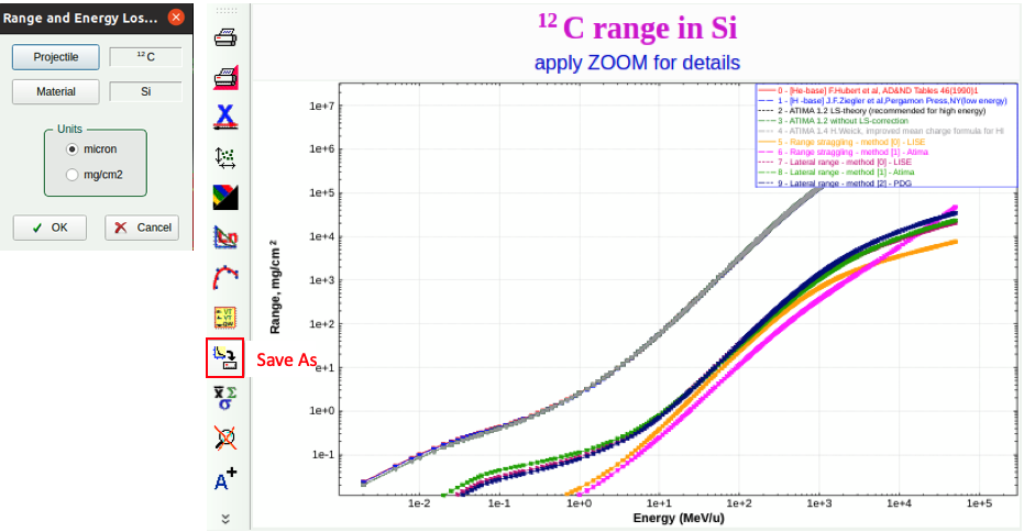
In this example, the $dE/dx$ and range data are taken from LISE++.
Reference:
LISE++ documentation:
https://lise.nscl.msu.edu/documentation.html
In LISE++, the relevant tools are:
Utilities -> Plots: Energy loss, Ranges ...Range in material ...Stopping power (dE/dx) ...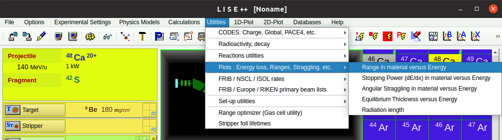
Choose the incident ion and material, then save the table to a text file.
2 Read LISE data into a TGraph
The LISE file provides energy in MeV/u and range in $\mu$m.
We read the table and store it as a TGraph:
- x-axis: Energy per nucleon $(\mathrm{MeV/u})$
- y-axis: Range $(\mu\mathrm{m})$
TGraph* ReadLiseRangeFile(const char* inputFile)
{
    ifstream inFile(inputFile);
    if(!(inFile.is_open())) {
        cout << "Cannot find input file : " << inputFile << endl;
        return 0;
    }

    TGraph *gER = new TGraph;
    string str;

    for(int i=0; i<3; i++)
        getline(inFile, str); // skip header lines

    // energy: MeV/u, Range: micron
    double energy, R[10], dummy;
    int n = 0;

    while(getline(inFile, str))
    {
        stringstream ss(str);
        ss >> energy >> R[0]
           >> dummy  >> R[1]
           >> dummy  >> R[2]
           >> dummy  >> R[3]
           >> dummy  >> R[4]
           >> dummy  >> R[5]
           >> dummy  >> R[6]
           >> dummy  >> R[7]
           >> dummy  >> R[8]
           >> dummy  >> R[9];

        gER->SetPoint(n++, energy, R[4]);
    }

    inFile.close();

    cout << "Read " << n << " lines of data from the file: " << inputFile << endl;
    cout << "TGraph: x = E(MeV/u), y = Range(um)" << endl;

    return gER;
}
Example:
TGraph *gER = ReadLiseRangeFile("12C-range.txt");
Read 268 lines of data from the file: 12C-range.txt
TGraph: x = E(MeV/u), y = Range(um)
3 Range curve of $^{12}\mathrm{C}$ in silicon
To visualize the range–energy relation, we define a small helper function for arrows and labels:
void draw(double x0, double y0, double x1, double y1,
          double tx0, double ty0, TString txt)
{
    TArrow *arrow = new TArrow(x0, y0, x1, y1, 0.005);
    TLatex *tex   = new TLatex(tx0, ty0, txt);

    arrow->SetLineColor(kBlue);
    arrow->SetLineStyle(2);
    arrow->Draw();

    tex->SetTextFont(13);
    tex->SetTextSize(15);
    tex->SetTextAlign(12);
    tex->SetTextAngle(0);
    tex->SetTextColor(kRed);
    tex->Draw();
}
Now draw the graph:
TCanvas *c1 = new TCanvas("c1","c1",800,600);

gER->SetTitle("Range vs Energy; MeV/u; um");
gER->SetLineColor(kBlue);
gER->SetMarkerColorAlpha(kRed, 0.2);
gER->Draw("AL*");

draw(40, 0, 40, gER->Eval(40), 40, 0.02, "E_{0}");
draw(20, 0, 20, gER->Eval(20), 20, 0.02, "E_{1}");

draw(0, gER->Eval(40), 40, gER->Eval(40), 1.0e-4, gER->Eval(40), "R(E_{0})");
draw(0, gER->Eval(20), 20, gER->Eval(20), 1.0e-4, gER->Eval(20), "R(E_{1})");

c1->SetLogx();
c1->SetLogy();
c1->Draw();
This graph is the basis for the residual-range calculation below.
4 Energy-loss calculation by the residual-range method
Suppose a particle enters silicon with initial energy $E_0$ and passes through thickness $\Delta x$.
Step 1: Convert energy to range
From the graph:
$$ R_0 = R(E_0) $$
In ROOT:
double R0 = gER->Eval(E0, 0, "S");
Step 2: Subtract the detector thickness
After crossing material thickness $\Delta x$, the residual range is
$$ R_1 = R_0 - \Delta x $$
Step 3: Convert residual range back to energy
We need the inverse function $E(R)$.
Since gER is $R(E)$, we build a new graph by swapping x and y:
TGraph *gRE = new TGraph(gER->GetN(), gER->GetY(), gER->GetX());
Then the remaining energy is
$$ E_1 = E(R_1) $$
In ROOT:
double E1 = gRE->Eval(R1, 0, "S");
Step 4: Compute energy loss
Finally,
$$ \Delta E = E_0 - E_1 $$
5 Example: 200 MeV $^{12}\mathrm{C}$ through 300 $\mu$m silicon
A subtle but important point: the LISE table uses MeV/u, while the beam energy here is given as total energy in MeV.
For $^{12}\mathrm{C}$ with mass number $A=12$,
$$ E/A = \frac{200}{12} \text{ MeV/u} $$
So the range must be evaluated using $E/A$, not the total energy.
int A = 12;
double dx = 300;   // um
double E0 = 200.;  // total MeV
double dE;

double R0 = gER->Eval(E0/A, 0, "S");
TGraph *gRE = new TGraph(gER->GetN(), gER->GetY(), gER->GetX());

cout <<"R0 = "<< R0 << "um" << endl;

if(R0 > dx) {
    double R1 = R0 - dx;
    double E1_A = gRE->Eval(R1, 0, "S");  // remaining energy per nucleon
    dE = E0 - E1_A*A;                     // convert back to total energy
}
else {
    dE = E0; // particle stops in detector
}

cout << "Energy loss of " << E0 << " MeV 12C in "
     << dx << " um Silicon: " << dE << " MeV" << endl;
R0 = 587.079um
Energy loss of 200 MeV 12C in 300 um Silicon: 69.3239 MeV
Interpretation
- Initial total energy: $200$ MeV
- Initial energy per nucleon: $16.67$ MeV/u
- Initial range: about $587~\mu$m
- After passing through $300~\mu$m of Si, the particle still exits the detector
- Estimated energy deposited in the detector: about $69.3$ MeV
This is physically reasonable.
6 A reusable energy-loss function
We now define a general function for the mean energy loss:
Input:
A: mass numberE0_A: initial energy per nucleon in MeV/udx: detector thickness in $\mu$mgER: graph of range vs energy per nucleon
Output:
- total energy loss in MeV
This is a convenient design, because the LISE table is naturally given in MeV/u.
double eloss(int A, double E0_A, double dx, TGraph *gER)
{
    double dE_A;
    double R0 = gER->Eval(E0_A, 0, "S");

    TGraph *gRE = new TGraph(gER->GetN(), gER->GetY(), gER->GetX());

    if(R0 > dx) {
        double R1   = R0 - dx;
        double E1_A = gRE->Eval(R1, 0, "S");
        dE_A = E0_A - E1_A;
    }
    else {
        dE_A = E0_A;
    }

    delete gRE;
    return dE_A * A;
}
Test:
cout << eloss(12, 200./12, 300, gER) << endl;
69.3239
Telescope: $\Delta E-E$
Now consider a three-layer silicon telescope:
- $E_1$: 100 $\mu$m
- $E_2$: 300 $\mu$m
- $E_3$: 2000 $\mu$m
These layers allow us to measure:
- $\Delta E_1$: energy loss in the first detector
- $\Delta E_2$: energy loss in the second detector
- $E$: residual energy deposited in the last detector
This is the standard basis of $\Delta E-E$ particle identification.
Minimum energy required to penetrate each detector
Using the inverse graph $E(R)$, we can estimate the minimum incident energy needed to cross a given detector thickness.
TGraph *gRE = new TGraph(gER->GetN(), gER->GetY(), gER->GetX());

cout << "Minimum energy required for penetrating detectors:" << endl;
cout << "E = " << gRE->Eval(100)*12  << " MeV for E1 detector." << endl;
cout << "E = " << gRE->Eval(300)*12  << " MeV for E2 detector." << endl;
cout << "E = " << gRE->Eval(2000)*12 << " MeV for E3 detector." << endl;
Minimum energy required for penetrating detectors:
E = 67.089 MeV for E1 detector.
E = 134.155 MeV for E2 detector.
E = 401.473 MeV for E3 detector.
7. Simulation
We now simulate $5\times10^5$ events.
Assumptions:
- incident ion: $^{12}\mathrm{C}$
- incident total energy: uniform from 0 to 500 MeV
- detector thicknesses:
- $t_1 = 100~\mu$m
- $t_2 = 300~\mu$m
- $t_3 = 2000~\mu$m
- detector resolution: $$ \sigma_E = 0.01\sqrt{E} $$
Histograms for the telescope response**
These histograms store:
h1,h2,h3: energy deposited in each detector layerh12: correlation between $E_2$ and $E_1$h23: correlation between $E_3$ and $E_2$h1all: correlation between total deposited energy and first-layer energy
The simulation sequence
For each event:
- Start with total energy $e$
- Compute energy loss in layer 1: $$ e_1 = \Delta E_1 $$
- Remaining energy after layer 1: $$ e - e_1 $$
- Use that remaining energy as the input for layer 2
- Repeat for layer 3
TH1F *h1    = new TH1F("h1",   "E1",      2000, -10, 500);
TH1F *h2    = new TH1F("h2",   "E2",      2000, -10, 500);
TH1F *h3    = new TH1F("h3",   "E3",      2000, -10, 500);

TH2F *h12   = new TH2F("h12",  "E1-E2",   2000, -10, 500, 600, -10, 150);
TH2F *h23   = new TH2F("h23",  "E2-E3",   2000, -10, 500, 600, -10, 150);
TH2F *h1all = new TH2F("h1all","E1-Eall", 2000, -10, 500, 600, -10, 150);

int A = 12;
double t1 = 100;
double t2 = 300;
double t3 = 2000;

for(int i=0; i<500000; i++) {
    double e = gRandom->Uniform(0, 500);

    double e1 = eloss(A, e/A,                 t1, gER);
    double e2 = eloss(A, (e-e1)/A,            t2, gER);
    double e3 = eloss(A, (e-e1-e2)/A,         t3, gER);

    e1 = gRandom->Gaus(e1, 0.01*sqrt(e1));
    e2 = gRandom->Gaus(e2, 0.01*sqrt(e2));
    e3 = gRandom->Gaus(e3, 0.01*sqrt(e3));

    h1->Fill(e1);
    h2->Fill(e2);
    h3->Fill(e3);

    h12->Fill(e2, e1);
    h23->Fill(e3, e2);
    h1all->Fill(e1+e2+e3, e1);

    if(i % 100000 == 0)
        cout << ".";
}
cout << endl;
.....
Simulation
- 加入探测器分辨,假设$\sigma_E=0.01*\sqrt{E}$
- 注:实际半导体探测器分辨远小于设置值。
int A = 12;
double t1 = 100;
double t2 = 300;
double t3 = 2000;

for(int i=0; i<500000; i++) {

    double e = gRandom->Uniform(0,500);
    double e1 = eloss(A,e/A,t1,gER);
    double e2 = eloss(A,(e-e1)/A,t2,gER);
    double e3 = eloss(A,(e-e1-e2)/A,t3,gER);

    e1 = gRandom->Gaus(e1, 0.01*sqrt(e1));
    e2 = gRandom->Gaus(e2, 0.01*sqrt(e2));
    e3 = gRandom->Gaus(e3, 0.01*sqrt(e3));

    h1->Fill(e1);
    h2->Fill(e2);
    h3->Fill(e3);

    h12->Fill(e2,e1);
    h23->Fill(e3,e2);
    h1all->Fill(e1+e2+e3,e1);

    if(i%100000 == 0)
        cout << "." ;
}
cout << endl;
.....
Draw the 1D spectra
These spectra show the deposited energy distributions in the three detectors.
TCanvas *c2 = new TCanvas("c2","c2",900,300);
c2->Divide(3,1);

c2->cd(1);
gPad->SetLogy();
h1->Draw();

c2->cd(2);
gPad->SetLogy();
h2->Draw();

c2->cd(3);
gPad->SetLogy();
h3->Draw();
c2->Draw();
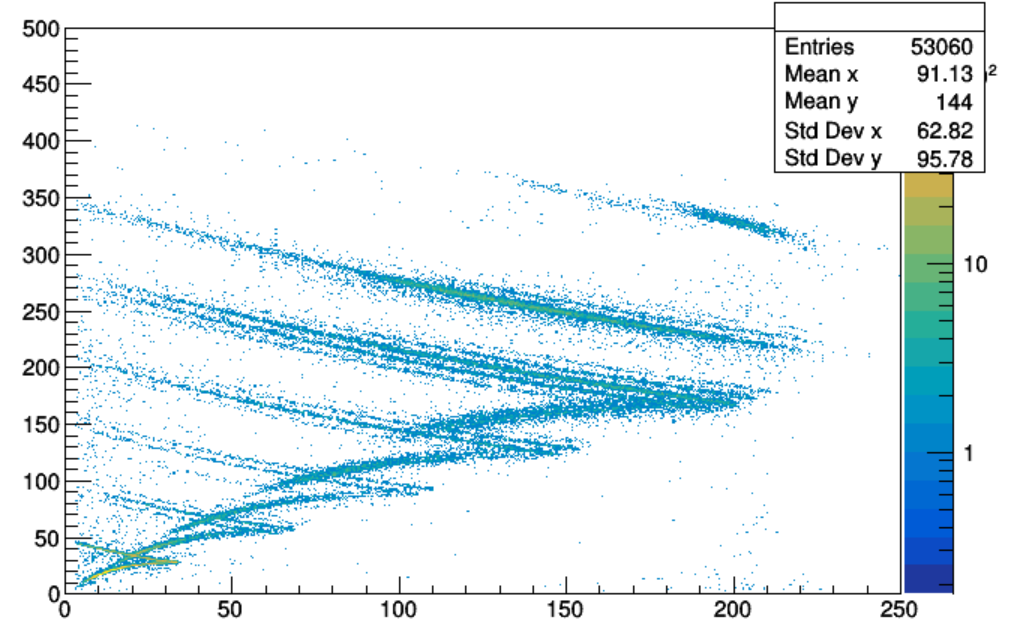
Draw the 2D $\Delta E-E$ plots
These two-dimensional plots are the basis for particle identification.
For a single isotope such as $^{12}\mathrm{C}$, the pattern is only one band.
When multiple isotopes are included, separate loci should appear.
TCanvas *c3 = new TCanvas("c3","c3",900,300);
c3->Divide(3,1);

c3->cd(1);
h12->Draw("colz");
gPad->SetLogz();

c3->cd(2);
h23->Draw("colz");
gPad->SetLogz();

c3->cd(3);
h1all->Draw("colz");
gPad->SetLogz();

c3->Draw();
Homework
Extend the simulation to several isotopes, for example:
- $^{7}\mathrm{Be},\ ^9\mathrm{Be},\ ^{10}\mathrm{Be}$
- $^{10}\mathrm{B},\ ^{11}\mathrm{B},\ ^{12}\mathrm{B}$
- $^{11}\mathrm{C},\ ^{12}\mathrm{C},\ ^{13}\mathrm{C},\ ^{14}\mathrm{C}$
Tasks
- Simulate each isotope in the energy range 0–300 MeV
- Generate 100000 events for each isotope
- Save the results into a TTree
- Analyze the tree in ROOT
Suggested branches
Store at least:
ZAe: incident total energye1: energy loss in detector 1e2: energy loss in detector 2e3: energy loss in detector 3
Suggested plots
Use ROOT to draw:
tree->Draw("e1:e2");
tree->Draw("e2:e3");
tree->Draw("e1:e1+e2+e3");
tree->Draw("e1:e");
- Expected Results:
Verification
Verify the relation between the $\Delta E-E$ two-dimensional plots and the particle species by applying different selection conditions in Draw(), for example with different values of $Z$ or $A$.
Example:
tree->Draw("e1:e2", "Z==6");
tree->Draw("e1:e2", "A==12");
tree->Draw("e1:e2", "Z==6 && A==12");
Check whether different isotopes or elements form different bands, and describe how the band positions change in the 2D plots.
Questions to think about
- How well are neighboring isotopes separated?
- Which detector combination gives the clearest PID bands?
- How does detector resolution affect the separation?
- What happens if you change detector thicknesses?
- For different particles, to which characteristic features in the 2D plots do the minimum incident energies required to penetrate the three detectors $\Delta E_1$, $\Delta E_2$, and $E$ correspond?
Hint
Compare the calculated penetration thresholds with visible features of the PID bands, such as their starting points, turning points, or boundaries in the $\Delta E-E$ spectra.